
arXiv:2207.09439v1 [cs.CC] 19 Jul 2022
All Paths Lead to Rome
Kevin Goergen, Henning Fernau, Esther Oest, Petra Wolf
∗
Universität Trier, Fachbereich 4 – Abteilung
Informatikwissenschaften
54286 Trier, Germany.
{s4kegoer,fernau,s4esmeck,wolfp}@uni-trier.de
Abstract
All roads lead to Rome is the core idea of the puzzle game Roma. It
is p layed on an n × n grid consisting of quadratic cells. Those cells are
grouped into boxes of at most four neighboring cells and are either filled,
or to be filled, with arrows pointing in cardinal directions. The goal of the
game is to fill the empty cells with arrows such t hat each box contains at
most one arrow of each direction and regardless where we start, if we follow
the arrows in the cells, we will always end up in the special Roma-cell.
In this work, we study the computational complexity of the puzzle game
Roma and show that completing a Roma board according to the rules is
an NP-complete task, counting the number of valid completions is #P-
complete, and determining the number of preset arrows needed to make
the instance uniquely solvable is Σ
P
2
-complete. We further show that the
problem of completing a given Roma instance on an n × n board cannot
be solved in time O
2
o(n)
under ETH and give a matching dynamic
programming algorithm based on the idea of Catalan structures.
1 Introduction
With computational devices in near ly everyone’s pockets nowadays, the oppor-
tunities to play puzzle games on these devices are plentiful. What makes such
games so addictive that they are played every day by millio ns of people? One
possible answer to the suggested question is that (generalized variants of) these
games are computationally intractable [12,30], which could explain why it can
be so challenging to find a solution or to get a g ood score. In this work, we study
the puzzle game Roma (a playable version can be found in [29]), which we de-
scribe in more detail in the next se ction. Roma has similarities to other puzzle
games, such as the famous Sudoku puzzle, shown to be NP-complete in [42],
in the sense that the player has to fill out fields in a two-dimensional board,
∗
Supported by Deutsche Forschungsgemeinschaft (DFG), project FE560/9-1.
1
taking into account hints and restrictions given by the concrete ins tance of the
game. Puzzle games of this sort such as Kakuro [37], Herugolf and Ma karo [27],
Dosun-Fuwari [28], or Ying-Ya ng puzzles [15] were shown to be NP-complete.
However, Roma is motivated by a concrete planning task : the player is asked
to design a map of one-way roads under certain restrictions so that finally, one
can travel to the central place (Rome) from each position on the map. Roma
can hence be used to explain the difficulties of planning and design in a playful
way.
The field of computational complexity of games and computer games is
a broad vivid field as it also allows a playful entry to the field of computa-
tional complexity theory, see for instance the surveys by Demaine et al. [12]
and K e ndall et al. [30]. T he importance o f the field is also reflected in a huge
number of publications at different international conferences over decades , such
as in the conferences JCDCG3 [1] and FUN [22]. The study of game s is not only
a fun topic but also allows fo r a deep e r understanding of fundamental concepts
in theore tical computer science. For instance, the game of cops and robbers
played on some graph G has a direct connection with the treewidth of G [5,38],
one of the mos t important structural pa rameters in parameterized complexity
theory. Further, game variants of problems can be used to study a problem
from a different perspective, for ins tance, a two-player variant o f the satisfia-
bility problem is equivalent to the PSPACE-complete quantified SAT problem
and can be even harder if we inherit rules native to the game Go [9, 35, 39].
Hence, studying (computer) games is a great way to better understand com-
binatorial concepts. In recent years, two notable lines of re search developed
in this field. One is trying to generalize the combinatorial key mechanics of a
game and studies the complexity of this combinatorial mechanics through so-
called metatheorems [13,14,20,23,40]. Another line of research focuses more o n
the individual games [2,7,11,21,34,36,41] and a lso takes a deeper analysis with
respect to parameterized complexity theory [3, 6,8, 19]. With this work, we are
going to contribute to the second line: we analyze the complexity of the game
Roma also from a parameterized angle.
Our contribution. We show that the question whether a partially filled in-
stance of Roma can be completed according to the rules of Roma is an NP-
complete problem by a r e ductio n from Planar 3SAT (Theorem 2). As this
reduction is parsimonious, we directly get that the counting variant of Roma,
counting the number o f solutions, is #P-complete (Theorem 10). The parsimo-
nious reduction further implies that the question of how many hints must be
added to a Roma instance in order to ma ke it uniquely solvable is Σ
P
2
complete
(Theorem 11). We show that the reduction by Lichtenstein [31] from 3SAT to
Planar 3SAT can be translated into our Roma s etting with only a constant
factor increase in space. Especially, we have that the number of va riables and
the number of clauses each correspond to the dimension n of an n × n Roma
board and hence, assuming ETH, Roma cannot be solved in time O
2
o(n)
(Theorem 9). As our second main result, we match this lower bound by a dy-
2
(0,0)
(0,1) (3,1)
(3,3)
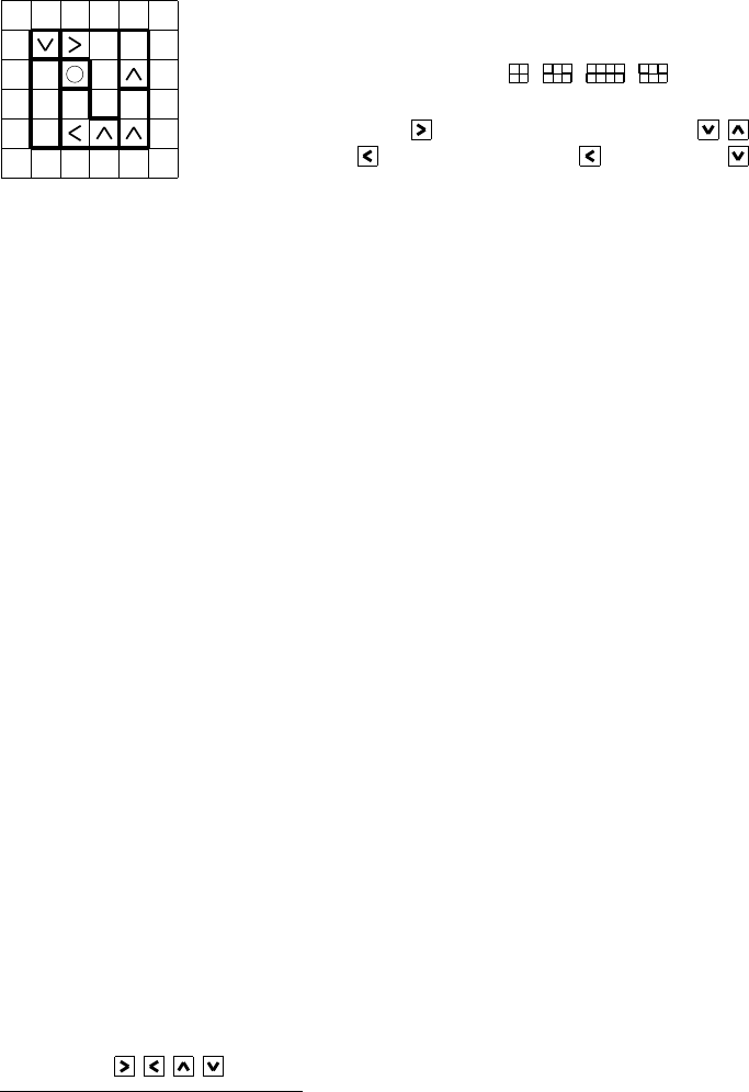
The indices explain how cells are a ddressed on the board.
Boxes are defined by drawing thicker b oundaries. Up to
symmetry, all different 2-boxes and 3-boxes ar e used. Ther e
are four other types of 4-boxes:
, , , . A typi-
cal reasoning is: Consider cell (3, 1). We cannot leave the
board, which excludes
. The preset 2-box excludes , .
Hence, ω(3, 1) = . Similarly, ω(3, 3) = , so ω(2, 3) = ,
etc.
Figure 1: Example of a 4 × 4 Roma game board, showing the ma in ingredients
of a Roma puzzle and its presentation throughout this paper.
namic programming alg orithm, we believe to be interesting, using the idea of
Catalan structures (Theorem 13).
The Rules of Roma
Roma is a one-person puzzle game. A Roma board consists of a quadr atic game
board, which in turn consists of n × n quadratic individual c ells. One of these
cells is a previously determined Roma-cell which serves as a tar get cell. Cells
which directly border on each other are called true neighbors.
1
Cells which a re
true neighbors c an be gathered in a collection called a box. These boxe s can
consist of 1 to 4 cells . The boxes ar e preset at the beginning of a game and
every cell is contained in one box. The boxes can take any form, as long as
every cell within a box c an be reached from any other c ell w ithin that box by
only tr aversing other cells from the same box, where traversal refers to single-
cell steps from one cell to one o f its true neighbors. The Roma-cell is always
contained in its own 1-box. Each empty cell must be filled by the player with an
arrow, pointing in one of the four cardinal directions. Cells can contain preset
arrows before the game starts. Each box can contain o nly one arrow pointing
in a given cardinal direction. The goal of the game is to fill each cell in such a
manner that, beginning in any cell within the board, following the arrows step
by step will always lead to the Roma-cell. An example game board may look as
displayed in Figure 1. A more mathematical desc ription of the game will follow
next.
2
A Derived Decision Problem
An instance of Roma R consists of an n × n grid of cells C with C = {c
i,j
|
i, j ∈ [n]}. The preset entries of the instance are defined by a partial function
ρ: C → {◦,
, , , }, where only one cell, the Roma-cell c
R
∈ C, can be
1
In cellular automata theory, this notion of neighborhood is known as von-Neumann-
neighborhood. In image processing, this resembles the notion of 4-connected pixels.
2
From here on, we will refer to the formal decision problem as Roma as opposed to the
game Roma.
3
assigned with ◦. We assume that |ρ
−1
(◦)| = 1 . This leaves a set E
R
of empty
cells, for which ρ is not defined. The boxes of an instance are given by a set B
R
and a total function β : C → B
R
, where only up to four cells can be sorted into
one box. For brevity, we call a box with c cells a c-box. A cell can only be sorted
into a non-empty box if it is a true neighbor of one of the cells alrea dy sorted into
that b ox. A solution to an instance is an ass ignment ω : C → {◦,
, , , },
which is a total function that coincides with ρ whenever ρ is defined and that
is valid in the sense described next.
From an assignment ω, we can derive a dire cted graph G(ω) = (V, E) as
follows: V = C. Let c
i,j
, c
ℓ,k
∈ V . There is a directed edge (c
i,j
, c
ℓ,k
) ∈ E if and
only if one of the following four conditions is satisfied:
• ℓ = i and k = j + 1 and ω(c
i,j
) = ; or: ℓ = i and k = j − 1 and
ω(c
i,j
) = ; or:
• ℓ = i + 1 and k = j and ω(c
i,j
) =
; or: ℓ = i − 1 and k = j and
ω(c
i,j
) = .
An as signment ω is c alled valid if the following two conditions are met:
Box condition. There is no box to w hich ω assigns the same arrow twice, or,
more formally:
∀c
i,j
, c
ℓ,k
∈ C : (c
i,j
6= c
ℓ,k
∧ β(c
i,j
) = β(c
ℓ,k
)) =⇒ ω(c
i,j
) 6= ω(c
ℓ,k
) .
Graph condition. G(ω) is acyclic, weakly connected and c ontains a unique
vertex of out-degree zero, namely c
R
.
In particular, the graph condition rules out assignments with ω(c
0,0
) =
,
bec ause then c
0,0
has out-degree zero, or with ω(c
0,0
) = and w ith ω(c
0,1
) = ,
bec ause then the graph would be neither acyclic nor we akly connected. We next
show that all paths lead to Rome if the formulated conditions are met.
Lemma 1. From each vertex, there is a unique directed path to c
R
.
Proof. As any assignment can define for any c
i,j
∈ V at most one c
ℓ,k
such
that (c
i,j
, c
ℓ,k
) ∈ E, each vertex has maximum out-degr e e of one. This already
implies that, from each vertex, there exists at most one directed path to c
R
.
The graph condition then tells us that indeed all vertices but the Roma-cell c
R
have out-degree exactly one. Let v
0
∈ V , v
0
6= c
R
, be arbitrary. As G(ω)
is weakly connected, there exists a sequence of vertices v
0
, v
1
, v
2
, . . . , v
k
with
v
k
= c
R
and, for each i = 1, . . . , k, either (v
i−1
, v
i
) ∈ E or (v
i
, v
i−1
) ∈ E (but
not both because of acyc licity). As v
k
has out-degree zero, (v
k−1
, v
k
) ∈ E. As
v
k−1
has out-degree one, (v
k−2
, v
k−1
) is enforced. This argument propagates
inductively, so that finally (v
i−1
, v
i
) ∈ E for all i = 1, . . . , k can be concluded,
i.e., there exists a directed path from v
0
to c
R
.
Given an instance R = (n, ρ, β) of Roma, the question is if there exists a
solution or not. If we want to explicitly mention the board dimensions, we
sp eak of an n × n-Roma puzzle.
4

Henceforth, we will refer to the information a bout an element of { , , , }
as a signal or flow, whereas “signal” describes an information which can be passed
on to another cell by utilizing the rules of Ro ma (for example the special rela-
tionship between cells contained within the s ame box) and “flow” describes the
path which is followed when moving one cell at a time in the direction the ar row
contained in each given cell points in. Each flow nee ds to end in the Roma-cell
in order for the assignment of an insta nce to be valid.
2 Computational Hardness Results
In this section, we present our first main result, which is the following one.
Theorem 2. Roma is NP-complete.
As each cell is filled by one out of four possible directions, a solution can be
described with at most 2n
2
bits for a concrete Roma puzzle with n × n cells.
Hence, Roma is in NP. The main part of the section is devoted to a proof s ketch
for its NP-hardness. At the end, we derive several other conclusions from the
sp ecific nature of the reduction.
Recall that Roma is played on an n × n board. The NP-ha rdness of the
Roma puzzle is proven by a reduction from Planar 3SAT. According to Licht-
enstein [31], a 3-SAT formula ϕ is planar if the gra ph G(ϕ) = (V, E) admits an
embedding in the plane, where V = X ∪ C, with X being the variables of ϕ
and C being its clauses, and E c ontains two types of edges: (a) incidence edges:
xc ∈ E if variable x occurs (either positive or negated) in clause c, (b) cycle
edges: G[X] is a cycle. Instances of Planar 3SAT are planar 3-SAT formulas.
It is worth mentioning that in Lichtenstein’s constr uction, the graph G(ϕ) is of
bounded degree as can be observed in Figure 8, where the crossover-gadget of
the construction is depicted.
We will show how to cons truct a Roma puzzle R(ϕ) from a given pla nar 3-
SAT for mula ϕ in polynomial time. This implicitly assumes a planar embedding
of the graph G(ϕ) = (V, E). The edges of G(ϕ) require the distribution of a
signal between the variable and clause gadgets that we describe below. As we
have to mo del these edges in a discretized fashion in R(ϕ), we need a simple
gadget that allows to turn signals by 90 degrees. By describing this gadget, it
should also be made cle ar what signal means in our construction. Note that
gadgets described in the following will be embedded in a bigge r Roma board,
hence arrows can leave the gadget. We will later take care of those arrows by
leading their flow to the Roma-cell.
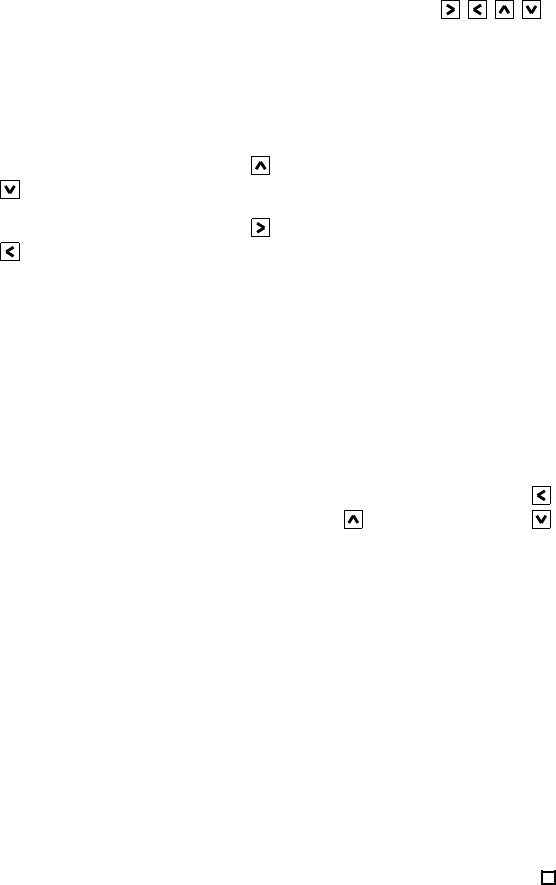
First, we create an L-shaped 4-box. In the context of this e xplanation, we set
the lower left cell of this box as c
0,0
with ρ(c
0,0
) =
and ρ(c
0,1
) = . This
5
means that β(c
0,0
) = β(c
0,1
) = β(c
0,2
) = β(c
1,0
) = b
0
. Then,
we create three additional boxes with β(c
2,0
) = b
1
; β(c
1,2
) = b
2
;
β(c
0,3
) = β(c
1,3
) = b
3
. Note that we may extend b
1
and b
3
to
contain additional cells if needed. Lastly, we set ρ(c
1,3
) =
and
ρ(c
1,2
) = . This gives the construction called corner-gadget,
depicted on the right. The cells showing their indices are still
to be set during a play. Note, that this gadget will be utilized
as part of the variable-gadget.
(1,0) (2,0)
(0,2)
(0,3)
Now and in the following, assume that ω is an assignment that resolves the
Roma puzzle, where this gadget is a piece of. We ca n show the following claim:
Lemma 3. (ω(c
2,0
) =
) implies (ω(c
0,3
) = ) and (ω(c
0,3
) = ) implies
(ω(c
1,0
) = ).
Hence, a path entering the g adget from the right lower end will cause an
upward direction at the upper left end, while a downward path at the upper
left end will c ause a right direction to be taken at the right lower end. We will
show-case the reasoning with this lemma , but rather only state claims below.
Proof. We need to prevent closed cycles, since otherwise there would be cells,
the flow of which would not reach the Roma-cell. This leads to:
(ω(c
2,0
) = ) → (ω(c
1,0
) = ) → (ω(c
0,2
) = ) → (ω(c
0,3
) = ) and
(ω(c
0,3
) = ) → (ω(c
0,2
) = ) → (ω(c
1,0
) = ). Further, ω(c
2,0
) 6= .
We also need to move a signal along in one direction. This can be done with
a straight-line gadget, described next.
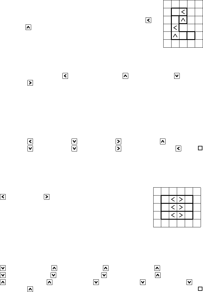
We create a 4-box, all cells of which are located in the same row. In the context
of this explana tion, we set the leftmost cell of this box as c
0,0
. This means that
β(c
0,0
) = β(c
1,0
) = β(c
2,0
) = β(c
3,0
) = b
0
. We set ω(c
1,0
) =
and ω(c
2,0
) = . A box such as this one will henceforth
be referred to a s a conductor-box. In order to complete our
gadget, we place two additional conductor-boxes on top of
the first one. The cells showing their indices are still to be
set during a play.
(0,0)
(0,1)
(0,2)
(3,0)
(3,1)
(3,2)
Lemma 4. If any cell in a straight-line gadget is validly assigned, there is only
one valid way to assign the other empty cells.
Proof. Assigning any cell within this gadget leads, by utilizing the rules of Roma,
to the following implications. W.l.o.g., we start by as signing c
0,0
: (ω(c
0,0
) =
) → (ω(c
3,0
) = ) → (ω(c
3,1
) = ) → (ω(c
3,2
) = ) → (ω(c
0,2
) =
) → (ω(c
0,1
) = ) → (ω(c
0,0
) = ) and (ω(c
0,0
) = ) → (ω(c
0,1
) =
) → (ω(c
0,2
) = ) → (ω(c
3,2
) = ) → (ω(c
3,1
) = ) → (ω(c
3,0
) = ) →
(ω(c
0,0
) =
).
By adding mo re conductor-boxes, s traight lines of arbitrary length can be
built. We a re now coming to the vertices of G(ϕ). As they also have higher de-
gree (although the degree can be always assumed to be bounded), we need some
6
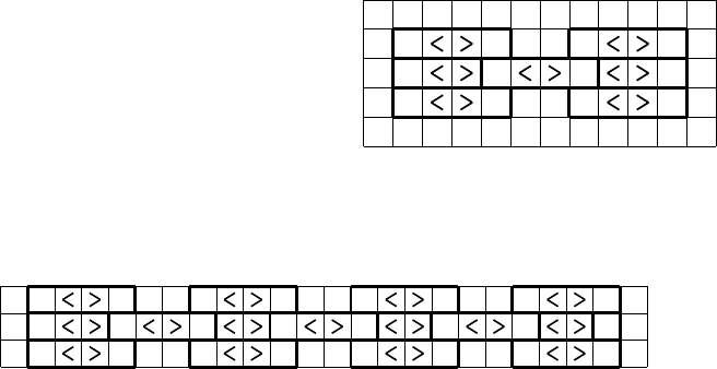
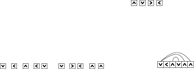
gadgets to fan signals out. We need to be able to fan a signal out in order to de-
liver
an information regarding a variable to
multiple gadge ts representing clauses con-
taining the said variable. This is done uti-
lizing the fanout-gadget displayed on the
right. It is based on the idea of stra ight-
line g adgets, so that we conclude:
(0,0)
(0,1)
(0,2)
(3,0)
(3,1)
(3,2)
(6,0)
(6,1)
(6,2)
(9,0)
(9,1)
(9,2)
Lemma 5. If any empty cell in a fanout-gadget is assigned, there is only one
valid way to assign the other empty cells.
Note that an arbitrary number of variations of fanout-gagdets can be con-
nected and utilized in order to transmit a signal horizontally:
So far, we mainly constructed geometric gadgets, but these are the building
blocks of the proper formula gadgets that we describe next. Let us mention one
more geometric detail: In G(ϕ), all vertices have been connected via a cycle. In
our construction, we actually only need a connection via a kind of path which we
refert to a s the core-line in the following. Next, we describe the logical gadgets,
which are gadgets for setting variables, literals and clause s.
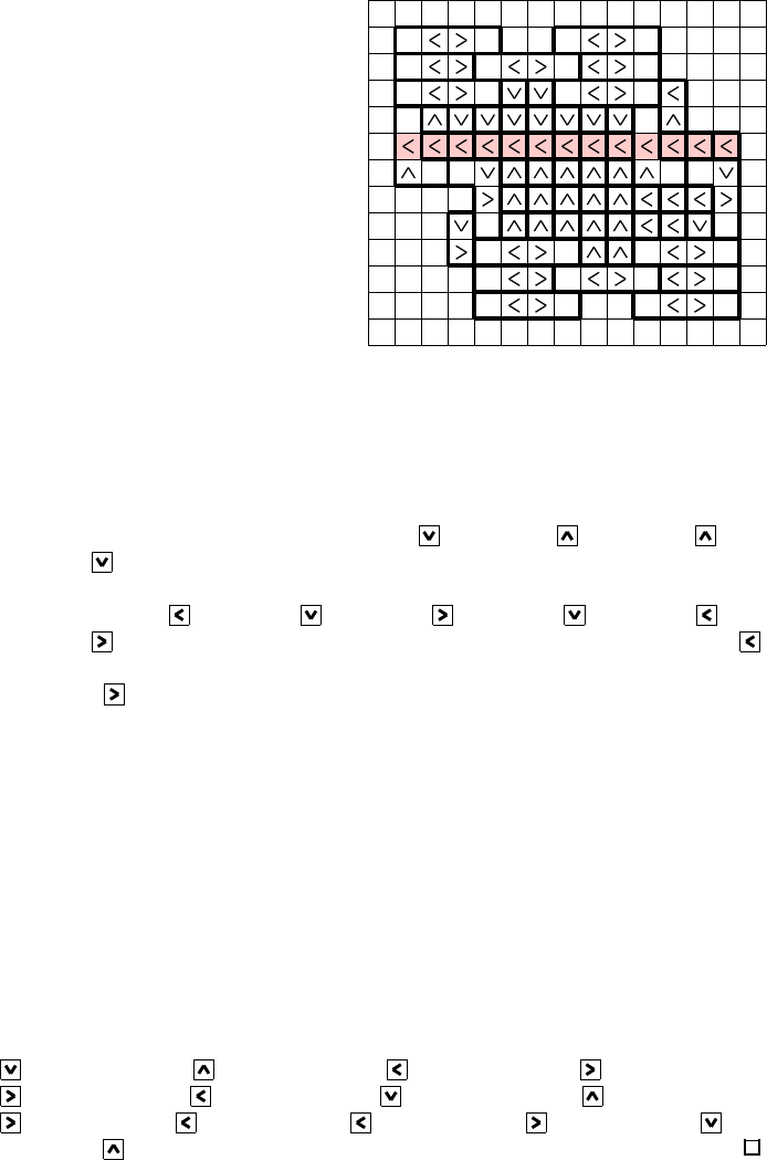
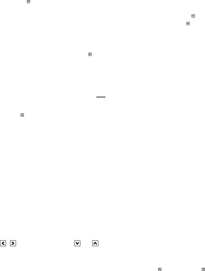
The variable-gadget is described in Figure 2. The picture c ontains quite a
number of preset 1-box cells in the middle, most of which are not necessary for
the g adgetry itself. Its sole purpo se is to form a proper Roma puzzle and to
guarantee that there is only one possible way to solve the Roma puzzle in case
the given Boolean formula was uniquely satisfiable. The essential preset cells
for the variable-gadget are shown in Figure 3. This gives s ome empty spac e,
but there is clearly far more empty space to be filled between the gadgets, when
we a ssemble the whole c onstruction of a given Boolean formula. How to fill this
space is explained in more details at the end of this section.
As the variable-gadget is built up from fanout- and corner-gadgets, the next
lemma follows directly from Theorem 3 and Theorem 5.
Lemma 6. If any empty cell in a variable-gadget is assigned, there is only one
valid way to assign the other empty cells.
As each cell within the variable-gadget can only be validly assig ned with one
of two options, the resulting two possibilities to assign the variable-gadget are
depicted in Figure 3. Clearly, the two options s hould correspond to setting the
variable true or false.
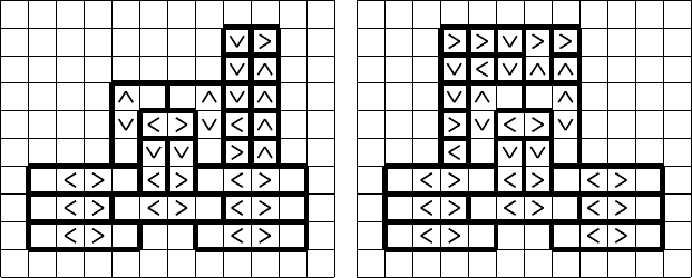
We need a gadget to represent the literals contained in clauses. Literals can
either be positive or negative. Positive literals ar e represented via the gadget
shown in Figure 4 on the left-hand side. We start the construction, once again,
with a fanout-gadget, which will ser ve as a connection for incoming straig ht-
line gadgets by placing it right below one of its bottom 4-boxes. Only one
7
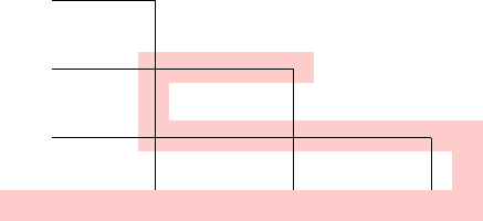
We start with a fanout-gadget at the bottom. Next, the lower left part of
this gadget will be connected to a modified corner-gadget, which does not
have the lower right 1-box as shown
above, and the top 2- box will be part
of the lower left 4-box of the fanout-
gadget instead. We now connect a
corner-gadget, modified in a slightly
different manner, to the lower right
part. Lastly, we co py this construc-
tion, rotate it by 180
◦
and connect
the two by connecting the loose ends
of the corner-gadgets, which allows
for additional 1-boxes to create a flow
from the right end of the gadget to its
left end as part of the core-line, high-
lighted in light red.
(0,0) (3,0) (6,0) (9,0) (12,0)
(3,1) (6,1) (9,1) (12,1)
(3,2) (6,2) (9,2) (12,2)
(3,3) (12,3)
(1,5) (2,5) (10,5)(11,5)
(0,7) (9,7)
(0,8) (3,8) (6,8) (9,8)
(0,9) (3,9) (6,9) (9,9)
(0,10) (3,10) (6,10) (9,10)
Figure 2: Variable-gadget with 1-boxes in the middle to form the core-line.
straight-line ga dget will be allowed to any given literal-gadget. We set the
bottom left cell of this fanout-gadget to be c
0,0
. Further more, we construct two
boxes with β(c
3,3
) = β(c
3,4
) = β(c
3,5
) = β(c
4,5
) = b
1
and β(c
5,5
) = β(c
6,5
) =
β(c
6,4
) = β(c
6,3
) = b
2
. We set ρ(c
3,4
) =
, ρ(c
3,5
) = , ρ(c
6,5
) = and
ρ(c
6,4
) = . The remaining cells encase d within the gadget are filled with three
boxes: β(c
4,2
) = β(c
4,3
) = b
3
, β(c
5,2
) = β(c
5,3
) = b
4
and β(c
4,4
) = β(c
5,4
) = b
5
.
We set ρ(c
4,2
) =
, ρ(c
4,3
) = , ρ(c
5,2
) = , ρ(c
5,3
) = , ρ(c
4,4
) = and
ρ(c
5,4
) = . Lastly, we place pre-filled 1-boxes as shown. Note that ω(c
6,3
) =
allows the flow coming from the 1-boxes to leave the gadget downwards, while
ω(c
6,3
) =
funnels it back into the rest o f the 1-boxes. This can be seen
by following the flow of the 1-boxes in Figure 4 and will be relevant when
constructing a clause-gadget.
Negative literals a re represented via the gadget displayed in Figur e 4 on the
right-hand side. We start the construction like the one for positive literals, but
instead of placing 10 1-boxes o n the right side, we use a somewhat different
design on the left side.
Lemma 7. If any empty cell in a literal-gadget is validly assigned, there is only
one valid way to assign the other empty cells.
Proof. We consider positive litera l-gadgets only; the proof for negative literal-
gadgets is analogous. The statement for the cells belonging to the fanout-
gadget follows from Theorem 5. The statement for c
3,3
, c
4,5
, c
5,5
and c
6,3
can be
shown by utilizing the rules of Roma. More precisely, we find: (ω(c
6,2
) =
) → (ω(c
3,2
) = ) → (ω(c
3,3
) = ) → (ω(c
4,5
) = ) → (ω(c
5,5
) =
) → (ω(c
6,3
) = ) → (ω(c
6,2
) = ) and (ω(c
6,2
) = ) → (ω(c
6,3
) =
) → (ω(c
5,5
) = ) → (ω(c
4,5
) = ) → (ω(c
3,3
) = ) → (ω(c
3,2
) = ) →
(ω(c
6,2
) =
).
8
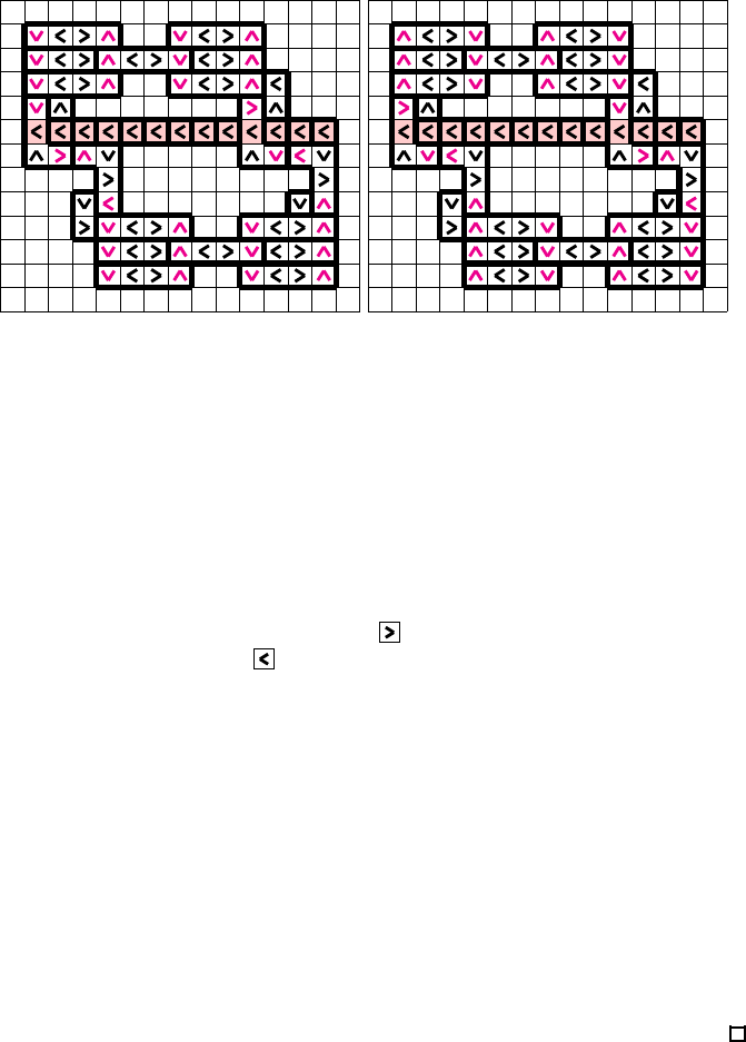
Figure 3: There a re exactly two ways to fill in the empty cells of the variable-
gadget. T he filled-in arrows on the left side are interpreted as setting the variable
to true, while the way the arrows are filled in on the right side should mean
that the variable is set to false. Note that this holds for both ways to fill in this
gadget and regardless of whether the connected clauses appear above or below
the core-line due to rotational symmetry of the fanout-gadgets used in both the
variable-gadgets as well as the literal-gadgets (see Figure 4).
The two p ossible valid as signments for negative literal-gadgets are shown in
Figure 5. Note that in this case ω(c
4,5
) =
funnels the flow back into the rest of
the 1-boxes, while ω(c
4,5
) = allows it to leave the gadget downwards, which is
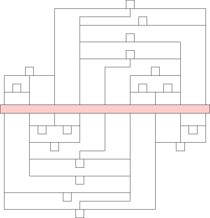
a b e havior opposite of positive literal-gadgets. In Figure 6, it is shown how the
literal gadgets are arranged to form a clause gadget. Clearly, the gadget can be
adapted to contain a n a rbitrary number of literals. Whether the literal-gadgets
represent positive or negative literals does not matter. W.l.o.g., we chose two
positive and one negative liter al for the demonstration of the clause-gadget. The
individual literal-gadgets are now connected through a cycle of 1-boxes.
Lemma 8. At least one literal-gadget within a clause-gadget needs to allow the
flow to leave the gadget downwards, or the assignment will be invalid.
Proof. If the flow is not allowed to leave the ga dget downwards through at
least one of its literal-gadgets, it is funneled back into the cycle of 1-boxes it
stems from. This holds true for both po sitive and negative literal-gadgets. If
every literal-gadget within a clause-gadget funnels it back an actua l flow-cycle
is crea ted, invalidating the overall assignment.
Since the lower part of the literal-gadget has the exact same structure as the
fanout-gadget, this part serves as a natural place to connect conductorboxes
which are part of fanout- or straightline-gadgets. Through this connection we
can propagate the assignment o f a connected variable-gadget. Note that the
part of the literal-gadget which resembles a fanout-gadget cannot be replaced
by a structure resembling a simple straight-line gadget a s this would destroy the
9
(0,0) (3,0) (6,0) (9,0)
(0,1) (3,1) (6,1) (9,1)
(0,2) (3,2) (6,2) (9,2)
(3,3) (6,3)
(4,5) (5,5)
(0,0) (3,0) (6,0) (9,0)
(0,1) (3,1) (6,1) (9,1)
(0,2) (3,2) (6,2) (9,2)
(3,3) (6,3)
(4,5) (5,5)
Figure 4: Variables may occur either positive (on the left) or negated (on the
right). This leads to slightly different shape s of the corresponding literal-gadgets
that form the basis of the clause-gadgets.
property of being a parsimonious reduction. Due to the ability of the fanout-
gadget to propagate the signal of one variable-gadget to multiple literal-gadgets,
we can check for each literal-gagdet, even for those belonging to different clause-
gadgets, whether the assignment of the c onnected variable-gadget allows the flow
of the literal- gadgets, and thus the clause-gadgets they are a part of, to reach
the Roma-cell and thus satisfy the clause. Even though each literal-gadget ends
up with two points which can connect to conductor boxes, it does not matter
whether the same variable is connected to both or just one of the same, as the
signal will be propagated either way. Two different variable-gadgets will not be
connected to the same literal-ga dget.
How exactly the individua l gadgets are connected is depicted in Figure 9,
where a small part of the crossover-gadget in Lichtenstein’s construction is real-
ized as a Roma board, e.g., variable-gadget γ is connected to literals from both
the gadgets of Clause 1 and Clause 2 utilizing straightline- and fanout-gadgets.
Finally, all variable gadgets will be connected via the core- line (as described
above), which will make it possible that all paths lead to the Roma- c ell, which is
placed on the leftmost cell of the core-line. Only a single cell within a variable-
gadget is assigned in or der to represent the assignment of the corresponding
variable. The resulting signal will be passed on to the connected literal-gadgets
in an unambiguous manner—after that firs t assignment, there is only one valid
assignment for the entire network consisting of a variable-gadget and straight-
line, fanout-, and literal-gadgets. Overall, there are only two valid ass ignments
for this network. The correctness of the overall construction fo llows by the
lemmas stated so far. Hence, the original 3-SAT formula ϕ has a satisfying
assignment if and only if the constructed Roma instance R(ϕ) has a so lution.
As can be seen in Figure 9, there are s till undefined cells between the con-
nected gadgets. Each of these cells will be prefilled and forms their own box.
At this point, it is important to realize that we can construct paths from ev-
ery single one of these cells either directly to the core-line, which leads to the
10
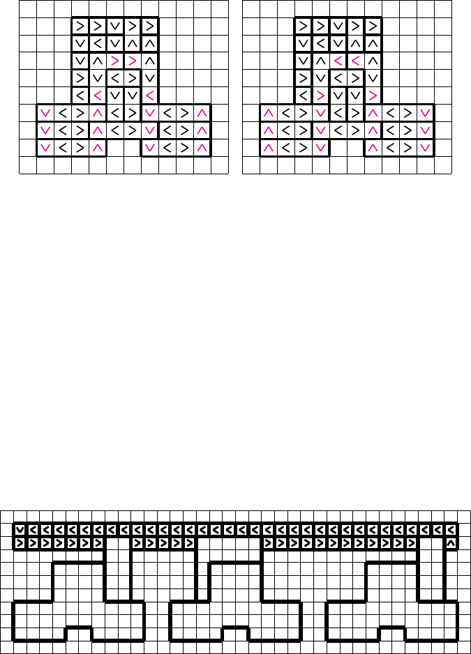
Figure 5: Negated literal-gadget filled in. The filled-in arrows on the left side
correspond to a true variable being connected to this gadget, in which case the
literal does not lead to satisfying the corresponding clause. When integrated
into a clause-gadget (see Figure 6) the upp e r two filled-in arrows will form a
closed cycle with the pres e t arrows, which leads to the Roma instance not being
valid. The filled-in arrows on the right side correspond to a false variable being
connected. In this case, the literal leads to the clause being satisfied by breaking
this closed cycle.
Roma-cell, or, in case of an encapsulated space , like the one between Clause 1
and Clause 2, to the upper part of a clause-gadget. I f we connect cells to a
clause-ga dget like that, the Roma-cell can be reached from all of these cells if
the corresponding c lause is satisfied in the same fashion as it can be reached
from the c e lls which are part of the gadget itself. Clearly, the very details of
the described filling of these boxes do not matter, it is only important that all
paths lead to Ro me.
Figure 6: Clause-gadget consisting of two positive and one negative literal.
11
a
b
c
C
1
C
2
C
3
Figure 7: As depicted in the construction by Lichtenstein 31 a planar embedding
of a 3SAT formula is shown where the variables are placed on a horizontal line
and the clauses are placed o n a vertical line. The variables are then connected
with the clauses in which they appear via rectangular lines . If those lines cross,
the crossing is replaced by a crossover-gadget, which is depicted in Figure 8.
The core-line connecting the varia bles with each other is depicted in red.
3 Further Complexity-Theoretic Consequences
In this section, we examine our reduction more carefully, so that we can deduce
several further interesting consequences. The first one deals with potential lim-
itations of exponential-time algorithms designed to solve a Roma instance, as
provided by the Exponential-Time Hypothesis, or ETH for short; see [26]. This
is interesting, as we will provide in the next section some matching algorithmic
results.
Theorem 9. Assuming ETH, there is no O
2
o(n)
-algorithm for solving n ×n-
Roma puzzles.
Proof. Here, we have to dig a bit deeper into the NP-hardness reduction o f
Lichtenstein [31]. He pres e nts a spec ific design that aligns all variables along
the x-axis and all clauses along the y-axis and then connects the variable to
the clauses that they are contained in by axes-parallel lines. Of course, these
straight lines will intersect, but he explains how to introduce crossover- gadgets
that will introduce a cons tant number of new variables and new clauses to
replace the crossings. We can first apply the famous sparsification lemma of
Impagliazzo and Paturi [26] to guarantee that the number of variables and the
number of clauses in the given 3-SAT formula are of the same order, say, N.
As there are at most N
2
crossings in the rectangular drawing, there will be no
more than O(N
2
) many variables and clauses in the instance of Planar 3SAT
that Lichtenstein proposes. Because each crossover-gadget can be simulated by
a network in a Roma instance that uses area O(1) only, see the Figur e s 7, 8,
and 9, we can build a Roma instance to the given 3SAT instance with at most
N variables and at most N clauses that is of size O(N
2
). Hence, if there was
an algorithm that would solve a n n × n-Roma puzzle in time O
2
o(n)
, then
one could solve any 3SAT instance with at most N variables and at most N
12

clauses in time O
2
o(N )
, contradicting ETH.
We now turn to a counting va riant of our main combinatorial problem:
#Roma is the problem to count the number of solutions of a Roma puzzle.
We might not like the idea tha t a given puzzle has too many solutions, as it
seems to be the case then that a human might find it awkward to play the game,
as seemingly not much cleverness is needed. This is why these puzzles are often
designed in a way that they admit only a unique solution. Still, counting the
number of solutions of a Ro ma puzzle is quite infeasible.
Theorem 10. #Roma is #P-complete.
Proof. As it is easy to design a Turing machine that first guesses an assignment
(a polynomial-size witness suffices by NP-membership) and then deterministi-
cally verifies the validity of it, we can also design a nondeterministic polynomial-
time Turing machine that has as many accepting paths as the original Roma
instance has solutions. Conversely, as the counting variant Planar #3SAT is
#P-complete [25] a nd the reduction from Planar 3SAT is pars imonious (this
can be checked by carefully going through the proofs of the previous lemmas
again), the number of satisfying assignments of this 3-SAT formula equa ls the
number of solutions of the constructed Roma instance.
Finally, for the design of uniquely solvable Roma puzzles, it would be good
to know how many hints have to be added (as preset arguments) to make a
puzzle uniquely solvable. We call this problem FCP Roma, to be spelled out
as Fewest Clues Problem. More formally, it is asked if there exist at most k
empty cells that can be assigned in such a manner that the remaining instance
only has a single valid assignment, given a Roma instance and an integer k as
inputs. This relates to FCP Planar 3SAT. Here, we are given a planar 3SAT
instance and an integer k, and it is asked if there exists a par tial assignment
of at most k variables such that the remaining formula has only one satisfying
assignment.
Theorem 11. FCP Roma is Σ
P
2
-complete.
Proof. We constructed an instance of Roma which is equivale nt to a given
instance of Planar 3SAT above. Ins tead of a partial assignment of k variables ,
we now assign k empty cells. For each assignment of a variable in the instance of
Planar 3SAT reduced from, we need to assig n exactly one cell in the resulting
instance of Roma, spe cifically one cell of the corresponding variable-gadget as
described above. Thus, the number of additional variables to be assigned k is
preserved. As FCP Planar 3SAT is Σ
P
2
-complete (see [16]), FCP Roma is
Σ
P
2
-hard. Conversely, in Section 3.1 of [16] it is s hown that the fewest clues
problem of every problem from NP is in Σ
P
2
.
After exhibiting these complexity-theoretic limitations of our problem, it is
interesting to see algorithms that can possibly meet the limitations. This is the
theme of the next section, where we first explain a rather simple branching algo-
rithm a nd then sketch a more sophisticated dynamic programming algorithm.
13

4 Algorithms for Solving Roma
A Search Tree Algorithm for Roma
Let n
2
be the total number of cells in a given instance of Roma R. Let k be
the number of empty cells in R. A first approach would test all possible four
assignments of each empty cell. This will, at worst, result in a running time
of O(4
k
· n
2
), because we have to check all n
2
cells to decide if the assignment
is valid or not for all 4
k
possible assignments. Naturally, this will be faster
the fewer empty cells R has. Overall the algorithm is polynomial in n and
exponential in k. This shows Roma to be fixed parameter tractable in the
standard parameter k. But can we do better? This will be examined in the
following.
Consider a ny c
ij
∈ E
R
. From a naive po int of view, there are 4 possible
assignments for c
ij
:
, , and . However, in many cases we can narrow
it down to a single a ssignment in polynomial time. Consider the following: We
start with all 4 possible assignments in mind. We then check the other cells of
box b
m
, which contains c
ij
. Each assignment already given within tha t box is
no longer an option fo r c
ij
. Next, we check each true neighbor of c
ij
. We follow
the flow of each of these cells. Should c
ij
pointing towards them lead to a clo sed
cycle (consisting of 2 cells or more ) this direction is not a n option for a valid
assignment. This includes borders of the board, since a rrows cannot point out
of the instance acc ording to the rules of Roma. If only one valid assignment is
left after these checks, we a ssign c
ij
, creating a new instance R
′
in the process,
and r ecurse our procedure with R
′
as input. In the worst case, no savings are
possible this way if we only consider boxes of size one. However, we get better
estimates in other cases.
Lemma 12. If R is an n × n-Roma puzzle with k empty cells, but without
empty cells that form 1-boxes, then R can be solved in time O(3.32
k
· n
2
).
Proof. The worst case clearly happe ns with 2-boxes now. Let b = {c
i,j
, c
i
′
,j
′
} be
a 2-box. If one of the two cells is pre-set, then we have at most three possibilities
for the empty cell. Otherwise, we find four possibilities for setting ω(c
i,j
). In
the three cases where ω(c
i,j
) does not point to c
i
′
,j
′
, we have each time three
possibilities for setting ω(c
i
′
,j
′
). In the case where ω(c
i,j
) points towards c
i
′
,j
′
,
only two possibilities remain for ω(c
i
′
,j
′
). Hence, altogether we have (at most)
11 possibilities to set ω on b, which is
√
11 ≤ 3.32 per cell.
Further improve ments are possible if there are only few 2-boxes and no 1-
boxes, but we refrain from giving further details here, because s till, k is of the
order of n
2
if we assume that relatively few hints are given at the beginning.
Therefore, the approach presented in the next subsection is (at lea st theoreti-
cally) more interesting.
A Dynamic-Programming Algorithm for Roma
We can get an algorithm that matches the lower bound of Theorem 9.
14
Theorem 13. There is an O
2
O(n)
-algorithm solving an n ×n -Roma puzzle.
The algorithm is based on a dynamic programming (DP) approach along the
rows of a Roma puzzle board. The main difficulty in obtaining the claimed run-
time bounds consists in the problem to check the graph condition of acyclicity.
A naive approach would end up with a run-time of O
2
O(n
2
)
, as a natural
idea would be to memorize for every pair of cells on the ‘sweep row’ (as we will
call the current row) whether or not a path leads from one cell to the other
through the already processed area of the board. To overcome this difficulty, we
make use of Catalan str uctur e s, similarly as pr oposed in [4,17] for quite different
problems on planar graphs that deal with c onnectivity co nstraints. As the name
suggests, these structures are related to a proper bracketing that models the
paths finally leading to the Roma-cell. We develop a special syntax for these
bracket structures to reflect their meaning with respect to configurations of the
Roma game.
Proof. The basic idea of the algorithm is to us e dynamic programming (DP)
along the rows of a Roma puzzle board. This sliding row works similar as a
sweep line in computational geometry, steadily moving downwards. We will
therefore speak about the (current) sweep row and the successor row. To each
row with n squares, we associate a string o f length at most 3n ove r the alphabet
Σ = ∆ ∪ ∆ × ∆ ∪ ∆ ×
∆
2
∪ B, where ∆ = {◦,
, , , } is the alphabet
of Roma cell states, and B = {[, ]} are brackets. We can formulate further
restrictions that would reduce the number of configurations considerably, but
we refrain from giving these details here, as they are immaterial to the claim.
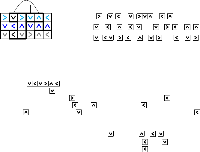
Let us explain the meaning of such a word encoding a row configuration by an
example for n = 6:
, { , }
, { , }
refers to the row
(1)
but encodes much more information. It also tells the box information that is
not shown in this picture, but that is important to keep from the previous rows,
stored in an abstr act fashion. This information is necessary to compute all
configurations of the succ e ssor row.
• A symbol from ∆ means, in the first place, that this symbol is sitting in
that cell of the sweep row. Besides this, it can encode two different things:
either the box of this cell is not continued in the successor row (in which
case we say that the symbol is of type 0), or this is the only symbol already
fixed for the box (i.e., this box was started on the sweep row), in which
case we say that the symbol is of typ e 3. Which of the two cases occurs
can be decided by the DP algo rithm by checking the given puzzle board.
• A symbol (a, b) ∈ ∆ × ∆ says: (1) Symbol a is in that cell of the sweep
row. (2) Because the box of this cell continues in the succes sor row, b is
15
the only symbol that is still available in that box. We also say that the
combined symbol (a, b) is of type 1.
• A symbol (a, {b, c}) ∈ ∆ ×
∆
2
means: (1) Symbol a is in that cell of the
sweep row. (2) The box of this cell continues in the successor row and
possibly beyond, and b , c are the symbols tha t are still available in that
box. We also say that the combined sy mbol (a, {b, c}) ∈ ∆ ×
∆
2
is of
type 2.
Using formal language terminology, from a row configuration w ∈ Σ
∗
, the row
content w
′
∈ ∆
∗
can b e retrieved by a morphism h which maps brackets to the
empty word, projects (a, x) 7→ a for (a, x) ∈ ∆ ×∆ ∪∆ ×
∆
2
and works as the
identity on ∆; see our example. A type that is bigger than zero tells the number
of possibilities that are still available for the remaining cells of that box. In a
sense, type 0 is an exception, as obviously no information has to be transferre d
into a “fresh row”.
To understand how updates in the DP procedure could work, we continue
with our example, see Figure 10. In order to describe how the next row could
be formed, we have to display a bit more of the board. The light blue first row
is showing only one possibility of how the previous row (with respect to the
sweep row in dark blue) could look like, not everything is enfo rced or known at
this step. In the last row, a possible success or row is indicated in gray, although
the two first gray arrows are enforced by the sweep row. The black arrows were
given as hints in the very beginning.
With
possible
bracket
structure
, { , }
,
, { , }
, { , }
,
, { , }
, { , }
Figure 10: The sweep row inherits information from its predecessor and passes
it to its succe ssor.
How does a successor row arrow consistency check work? We are considering
the string
∈ D
6
as a possible successor, one of many that we have
to check. The first is possible, as this starts a new box. Note that this is the
only choice for this cell, as would contradict with the pre-set in the second
cell, and further neither of
nor are possible, as is pointing to the left
wall and would contradict on the sweep row above. The next symbol is
given in the beginning. The symbol above on the sweep row does no t contradict
with this preset hint. As the box is finished in this row, the symbol has no
second component. The third symbol is
; it sees
, { , }
above, which
means that in the current box, the only symbols are
and that could be
put into the cell cur rently considered. But as left to it
was fixed, the symbol
16
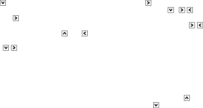
is indeed enforced. As the fourth symbol, we chose . Again, the box was
already considered in the sweep row, and the symbol above was
, { , }
, so
that
is one of the two possibilities. Howe ver, as the box is further continued
beyond the successor row, we have to introduce the combined symbol
,
.
The last two symbols,
and , are both in the same (new) box and hence
not c onflicting the sweep row above. However, they get a second component
{
, } to propagate the possibilities for the 4-box that will be completed in
the next row. The reader may check that also the predecessor row of the sweep
row is arrow-consistent with the sweep row.
We are now describing the role of the bracket structure that has to be used
in the successor row cycle consistency check explained below. This is imp ortant
as we have to prevent directed cyc le s in a c onstructed solution. We are first
assuming that the Roma-cell is not in the upper (‘forgotten’) part of the board.
This means that every path that enters the upper zone via a symbol
in the
sweep row must leave the upper zone again via a symbol
in the sweep row.
How exactly this pa th goes through the upp e r part is not important. Howe ver,
one can imagine these paths as for ming a kind of river system. Planarity ensures
that these paths never cross, but they could merge. Continuing with the ana logy,
one could try to draw some river basins. This is how one could interpret the
drawings of the lines in the pictures. In the sweep row picture in (1), the
rightmost upward arrow sta rts a path that goes all way along down again to
the first downward arrow. The penultimate upward arrow again starts a river
that flows (to stay in the picture) to the North-West, turning South again to
leave the area again via the first downward arrow . However, the first upward
arrow starts a river that flows to the North-East before turning So uth again to
leave the upward area via the second downward arrow. The role of the brackets
is to des c ribe these river basins in a unique way. In our example, the fir st pa th
that we described corresponds to the outermost matching pair o f brackets. How
is this constructed? The upward arrow points North-West, and this lets us
insert a closing bracket to the right of the upward arrow symbol. The matching
opening bracket is inserted to the right of the downward arrow that indicates
where this path leaves the upper part again. To formulate this bracket setting
rule more explicitly: Bra ckets are set to include the upward arrows (where the
river starts) but excludes the downward arrow (where the mouth of the river
is). The reason behind this convention of excluding the downward a rrows from
the brackets is that there might be rivers that start in the upper part but
share a mouth with a river that actually starts a t the sweep row. Furthermore,
downward arrows could receive paths from two directions, and it would destroy
the meaning of the bracket structure if we would have an opening bracket to the
left of a downward arrow and a closing bracket to its right. The second path
starts at the penultimate upward arrow, so we ins e rt a closing bracket to the
right of the upward arrow symbol. We insert the matching opening bracket to
the right of the downward arrow that indicates where this path leaves the upper
part again. Finally, the innermost pair of brackets indicates a flow from the first
upward a rrow to the North-East. Therefore, an opening bracket is inserted to
17
the left of this upward arrow, and we inser t a matching closing bracket to the
left of the downward arrow. Our conventions also imply that for each upwa rd
arrow, we have a pair of brackets, either with the opening bracket sitting to the
left of the upward arrow, or with the closing br acket sitting to the right of the
upward a rrow, while for the downward arrows, it could be the case that there
is no bracket attached to it (which means that these river s do not start at the
sweep row), or that even s e veral brackets are attached to it. Notice that closing
brackets are always sitting immediately to the left of a downward arrow, while
opening brackets are sitting to the right of a downward a rrow.
Let us add one further tho ught about the brackets: If we have, say, two
paths that start at the beginning of a row and move somehow through the
upper part of the board, to come down in two different downward arrows, then
it cannot be the case that the first path ends at the penultimate downward
arrow, while the second path ends at the last downward arrow, because this
would mean that these two paths have crossed, which is impossible as the overall
structure is planar. Similar ideas have been exploited implicitly in [4, 17]; the
so-called Catalan structures are referring to our explicit bracketings which catch
these ideas in a transparent way. We will exploit these connections ag ain when
counting the possible configurations below.
The successor row cycle consistency check will do two main things. Obvi-
ously, a successor row has to be rejected if it closes a path through the upper
part. Moreover, a ny bracket structure in a sweep row that is o therwise consis-
tent w ith the currently considered successor row induces a bracket structure on
the successor row in a unique manner. Let us describe this last point with our
example again. In the board picture of Figure 10, we see the bracket structure
and a ske tch of the corresponding river basin of the predecessor row. There is
only one path starting at the only upward arrow of that row, going North-Wes t
and e ntering that row again at a pre-set downward arrow. This is supposed to
be the path information that was propagated to the sweep row in the following
manner: For each upward arrow of the sweep row, we checked where it leads to
in the previous row. For instance, the last upward arrow points to a left arrow;
following this further (at the time when we constructed this config uration of
what is now the sweep row, the predecessor row was known to full extent), we
encounter an upward arrow who se matching downward arrow hap pens to be
pre-set. This path moves down to the sweep r ow and on the sweep row, the
left arrow moves to a nother downward arrow. Hence, we can draw this path (as
shown in the sweep row picture in (1)) from the rightmost to the leftmost cell of
the sweep row. The other connections are determined in an analogous fashion.
The reader is invited to also check the bracket structure of the successor row,
which again consists of a single pair o f brackets only.
This description should suffice to explain how to forma lly prove the claim
by induction.
However, notice that there could be several sweep row configurations that
are compatible with one string describing the cell contents of the successor
row. Therefore, there could be several different bracket structures that can be
associated to such a string over the alphabet ∆.
18
In o rder to count the possible configurations, we will go step-by-step.
First, a ssume that we consider a fixed bracket structure, and we also fixed for
each bracket pair which of the two brackets (opening or closing) is associated to
an upwar d arrow. In case we have combined symbols, we o nly consider whether
the first c omponent contains an upward arrow. Assume we have n
[ ]
bracket
pairs involved (as we see this many upward arrows on the sweep row) and that
we have n
[ ]
downward arrows that could be matched with these brackets on the
sweep row.
As the bracket structure is fixed, there are no more than
n
[ ]
+n
[ ]
n
[ ]
many
possibilities for such a matching. (In fa ct, there are less, as the bracket structure
is neglected in this type of counting, but we are not optimizing the counting
here.)
Next, assume that we have n
[ ]
upward arrows that are involved in potential
cycles. Recall that if the Roma-cell is in the upper part of the board, then not all
upward arrows need to be in a path tha t returns to the sweep row. As each such
upward arrow gives rise to a bracket pair, we only have to decide if the opening
or closing bracke t of this bracket pair is associated to such an upward arrow . It
is well-known that the number of ways we can properly form bracket expressions
with p pairs of brackets is given by
1
p+1
2p
p
, which is upper-bounded by 4
p
(this
is also known as Catalan numbe rs; see, e.g., Chapter 14 in [32]). Therefore, we
have 8
n
[ ]
many possibilities to cre ate bracket structures and fix the association
to upward arrows.
Next, we have to reason a bit about the type of the letters from ∆ and
how to count them. As the Roma-cell is unique and pre-set, this does not
enter the following consider ations. Recall that the type of a letter is completely
determined by the given box structure. Therefore, when we consider the set of
configurations of the sweep row, each cell may host different letters, but all of
them have the same type. Clearly, there are only 4 different letters of type 0
and of type 3. Ther e are 12 different combined letters of type 1, because the
combined letters (a, a ) ∈ ∆ × ∆ would never appear, as it makes no s ense to
put the symbol a into a cell and tell, at the same time, tha t the last symbol
that could be set in that box is also a. Similarly, there are also 12 different
combined letters of type 2, bec ause when we put a into the cell itself, there are
only
3
2
= 3 many possibilities to select two symbols from the 3 remaining ones.
In the worst case, this gives a factor of 3 for each of the 4 basic letters, which
corresponds to the factor 3
n
in (2).
Looking at a row with n cells, we can associate to each cell one of the letters
, or one of the states
′
or
′
, referring to downward or upward arrows
that are not invo lved in (potential) cycles. Altogether, this gives us the following
count for the number of configurations and hence for the space consumption of
our DP algorithm; for reasons of readability, we set k = n
[ ]
and t = k + n
[ ]
.
3
n
n
X
t=0
n
t
4
n−t
t
X
k=0
t
k
8
k
!
= 3
n
n
X
t=0
n
t
4
n−t
9
t
= 3
n
13
n
= 39
n
. (2)
19

For the update from one swee p row to the next, we need to cycle through
the (only) 4
n
‘new words’, comparing them against the (at most) 39
n
many
configurations of the ‘old sweep row’. Namely, the type of a letter is determined
from the box structur e . Altogether, this shows the claim of the theorem. Again,
we could optimize the counting of the running time, because there is a trade-off
between the types and the degree of freedom, but this would not change the
overall result.
5 Discussion
Games often come with some sort of dida c tical message. In o ur case, it is not
hard to s e e the Roma puzzle, being defined as a board game, to be g eneralizable
to a g ame on graphs. In other words, one could imagine this to b e a gentle
introduction into graph-theoretic concepts. The game Generalized Roma that
we propose is played on a weakly connected directed graph G
R
= (V, E) with a
sp ecial vertex c
R
, the Roma-vertex, having out-degree zero. More over, there is
a set of hints H ⊆ E. The task is to delete edges (not from the hints H) so that
the resulting graph is a directed acyclic graph that is weakly connected and has
maximum out-degree one. This could act as an introduction to graph-theoretic
notions like spanning trees or feedback arc sets. The proof of Theorem 1 is also
valid in this setting; this means again that all paths lead to Rome. So far, the
box condition has been neglected. This can be modeled as foll ows. We introduce
colors to the possible different orientations of each edge, i.e., we have a mapping
χ
E
: E → C
E
for the set of edge colors C
E
; also, we assign colors to ve rtices by a
mapping χ
V
: V → C
V
. Then, the box condition says that for each vertex color
c ∈ C
V
, the set of vertices χ
−1
V
(c) obeys that no two oriented edges e
1
, e
2
that
originate from vertices fro m χ
−1
V
(c) have the same color, i.e., χ
E
(e
1
) 6= χ
E
(e
2
).
This corresponds to having different arrows in the original Roma boxes. T his
generaliza tion would also a llow for another spec ialization and hence to different
game board designs. For instance, instead of taking quadratic cells (and hence
four directions for the arrows), one could also think of triangular ce lls (hence,
three directions for the arrows) or hexagonal c ells (with six directions for the
arrows); the box conditions would have to be adapted, too.
As an a lgorithmic challenge, it would be nice to further improve on the
algorithm pr oposed in Theorem 13. It is an open challenge to design alternative
algorithms tha t obtain running times within O
∗
(c
n
) for solving n × n-Roma
puzzles, best without using exponential space. Notice that our appro ach could
be also interpreted in terms of pathwidth, considering the ‘b oard gr aph’ that is
a grid. In this connection, we like to point to van der Zanden’s essay on puzzles
and treewidth [43]. There are other types of game problems where the same
challenge is ‘on the board’, for instance regarding finding a minimum dominating
set of queens on an n ×n chess board, see [18]. A possible way out to meet this
challenge could be to use the fact that planar graphs (e.g ., grid graphs) with n
2
vertices not only have treewidth of n, but also treedepth of n. Moreover, there
20
have been recent pap e rs [24, 33] that show that single-exponential algorithms
with parameter treedepth are possible for several problems , including those that
involve connectivity and cycle questions like Connected Vertex Cover and
Hamiltonian Cycle, and which use polynomial space only. We also refer
to the general discussions in [10]. In this direction, there would be also the
challenge to test different algorithmic approaches on concrete Roma puzzles,
including more standard approaches as using (I)LP s olver s.
21
a
1
γ
b
1
β ξ
δ
b
2
α
a
2
1
2
3 4
5
6
7
8
9
10
11
1213
14
15
16
17
18
Figure 8: Translation of the crossover-gadget replac ing crossings presented in
[31] for the setting of Roma. We connect variables b and b
2
as well as a and
a
2
, respectively, by utilizing straight-line gadgets, which saves us the trouble
of cr e ating clauses specifically to copy their assignments. The specific formula
reads, as presented in [31], as follows: (¬a
1
∨ ¬γ) ∧ (a
1
∨ b
1
∨ γ) ∧ (b
2
∨ ¬δ) ∧
(b
2
∨ ¬α) ∧ (¬δ ∨ ¬α) ∧ (α ∨ β ∨ ξ) ∧ (¬α ∨ ¬β) ∧ (a
2
∨ ¬β) ∧ (¬a
2
∨ b
1
∨ β) ∧
(a
2
∨ ¬α) ∧ (¬a
2
∨ ¬b
2
∨ α) ∧ (¬b
1
∨ ¬β) ∧ (¬b
1
∨ ¬γ) ∧ (¬β ∨ ¬γ) ∧ (γ ∨ δ ∨
¬ξ) ∧ (¬γ ∨ ¬δ) ∧ (¬a
1
∨ ¬δ) ∧ (a
1
∨ ¬b
2
∨ δ).
22
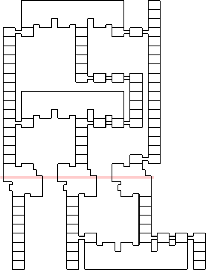
a
1
γ
b
1
Clause 1
Clause 2
Clause 13
Figure 9: Here we show a detailed Roma construction for a part of the gadget
shown above. Again, the co re-line is depicted in r e d. We connect var iables a
1
, γ
and a
2
to clauses 1, 2 and 13.
23
References
[1] Akiyama, J., Ito, H., Sakai, T., Uno, Y.: Twenty
years of progress of ${J C DCG}ˆ3$. Graphs Comb. 36(2),
181–203 (2020). https://doi.org/10.1007 /s00373-0 20-02133-4,
https://doi.org/10.1007/s00373-020-02133-4
[2] Almanza, M., Leucci, S., Panconesi, A.: Tracks from hell - when finding a
proof may be easier than checking it. In: Ito, H., Leonardi, S., Pagli, L.,
Prencipe, G. (eds.) 9th International Conference on Fun with Algo rithms,
FUN. LIPIcs, vol. 100, pp. 4:1–4:1 3. Schloss Dagstuhl - Leibniz-Zentrum
für Informatik (2018)
[3] Björklund, H., Sandberg, S., Vorobyov, S.: On fixed-parameter complex-
ity of infinite games. In: The Nordic Workshop on Programming Theory
(NWPT 2003). vol. 34 , pp. 29–31. Citese er (2003)
[4] Bodlaender, H.L., Cyg an, M., Kratsch, S., Nederlof, J .: Deterministic sin-
gle e xponential time algorithms for connectivity problems parameterized
by treewidth. Infor mation and Computation 243, 86–111 (2015)
[5] Bonato , A.: The game of cops and robbers o n graphs. American Mathe-
matical Society (2 011)
[6] Bonnet, É., Gaspers, S., Lambilliotte, A., Rümmele, S., Saffidine, A.: The
parameterized complexity of positional games. In: Chatzigiannakis, I., In-
dyk, P., Kuhn, F., Muscholl, A. (eds.) 44th International Colloquium on
Automata, Languages, and Programming, ICALP. LIPIcs, vol. 80, pp.
90:1–90:14. Schloss Dagstuhl - Leibniz-Zentrum für Informatik (2 017)
[7] Brunner, J., Chung, L., Demaine, E.D., Hendrickson, D.H., Hesterberg, A.,
Suhl, A., Zeff, A.: 1 X 1 rush hour with fixed blocks is PSPACE-complete.
In: Farach-Colton, M., Prencipe, G., Uehara, R. (eds.) 10th International
Conference on Fun with Algo rithms, FUN. LIPIcs, vol. 157, pp. 7:1–7:14.
Schloss Dagstuhl - Leibniz-Z e ntrum für Informatik (2021)
[8] Bruyère, V., Hautem, Q., Raskin, J.: Parameterized complexity of games
with mono tonically ordered omega-regular objectives. In: Schewe, S.,
Zhang, L. (eds.) 29th International Conference on Concurre ncy Theory,
CONCUR. LIPIcs, vol. 118, pp. 29:1–29:16. Schloss Dagstuhl - Leibniz-
Zentrum für Informatik (2018)
[9] Chandra, A.K., Kozen, D., Stockmeyer, L.J.: Alternation. Journal of the
ACM 28(1), 114–133 (1981)
[10] Chen, L., Reidl, F., Rossmanith, P., Villaamil, F.S.: Width, depth, and
space: Tradeoffs between branching and dynamic programming. Algo-
rithms 11(7), 98 (2018)
24
[11] Churchill, A., B iderman, S., Herrick, A.: Magic: The gathering is turing
complete. In: Farach-Colton, M., Prencipe, G., Uehara, R. (eds.) 10th
International Conference o n Fun with Algorithms, FUN. LIPIcs, vol. 157,
pp. 9:1–9:19. Schloss Dag stuhl - Leibniz-Zentrum für Informatik (2 021)
[12] Demaine, E.D.: Playing games with algorithms: Algorithmic combinatorial
game theor y. In: Sgall, J., Pultr, A., Kolman, P. (eds.) Mathematical Foun-
dations of Computer Science 2001, 26th International Symposium, MFCS.
Lecture Notes in Computer Science, vol. 2136, pp. 18–32. Spring er (2001)
[13] Demaine, E.D., Hearn, R.A.: Constraint logic: A uniform framework for
modeling computation as games. In: Proceedings of the 23rd Annual IEEE
Conference on Computational Complexity, CCC. pp. 149–162. IEEE Com-
puter Society (2008)
[14] Demaine, E.D., Lockhart, J., Lynch, J.: The computational complexity
of portal and other 3D video games. In: Ito, H., Leonardi, S., Pagli, L.,
Prencipe, G. (eds.) 9th International Conference on Fun with Algo rithms,
FUN. LIPIcs, vol. 100, pp. 19:1–19:22. Schloss Dagstuhl - Leibniz-Zentrum
für Informatik (2018)
[15] Demaine, E.D., Lynch, J., Rudoy, M., Uno, Y.: Yin-Yang puzzles are NP-
complete. In: He, M., Sheehy, D. (eds.) Proceedings of the 33rd C anadian
Conference o n Computational Geometry, CCCG. pp. 97–106 (2021)
[16] Demaine, E.D., Ma, F., Schvartzma n, A., Waingarten, E., Aaronson, S.:
The fewest clues problem. Theoretical Computer Science 748, 28–39 (2018)
[17] Dorn, F., Fomin, F.V., Thilikos, D.M.: Catalan structures and dynamic
programming in H-minor-free graphs. Jour nal of Computer and System
Sciences 78(5), 16 06–1622 (2012)
[18] Fernau, H.: minimum dominating set of queens: A trivial program-
ming exercise? Discrete Applied Mathematics 158, 308–318 (2010)
[19] Fernau, H., Hagerup, T., Nishimura, N., Ragde, P., Reinhardt, K.: On the
parameterized complexity of a generalized Rush Hour puzzle. In: Canadian
Conference o n Computational Geometry, CCCG 2003. pp. 6–9 (2003)
[20] Forisek, M.: Computational complexity of two-dimensional platform
games. In: Boldi, P., Gargano, L. (eds.) Fun with Algorithms, 5th Inter-
national Conference, FUN. Lecture Notes in Computer Science, vol. 6099,
pp. 214–227. Springer (2010)
[21] Fraenkel, A.S., Lichtenstein, D.: Computing a perfect strategy for n × n
chess re quires time e xponential in n. Journal of Combinatorial Theory,
Series A 31(2), 199–214 (1981)
25
[22] Fraigniaud, P., Uno, Y. (eds.): 11th International Conference on Fun with
Algorithms, FUN 2022, May 30 to June 3, 2022, Island of Favignana, Sicily,
Italy, LIPIcs, vol. 226. Schloss Dagstuhl - Leibniz-Z e ntrum für Informatik
(2022), https://www.dagstuhl.de/dagpub/978-3-95977-232-7
[23] de Haan, R., Wolf, P.: Restricted power - computational complexity results
for strategic defense games. In: Ito, H., L e onardi, S., Pagli, L., Prencipe, G.
(eds.) 9th International Conference on Fun with Algorithms, FUN. LIPIcs,
vol. 100, pp. 17:1–17:14. Schloss Dagstuhl - Leibniz-Zentrum für Informatik
(2018)
[24] Hegerfeld, F., Kratsch, S.: Solving connectivity problems parameterized by
treedepth in single-exponential time and polynomial space. In: Paul, C.,
Bläser, M. (eds.) 37th International Symposium on Theoretical Aspects
of Computer Science, STACS. LIPIcs, vol. 154, pp. 29:1–29:16. Schloss
Dagstuhl - Leibniz-Zentrum für Informatik (2020)
[25] Hunt, H.B., Mara the, M.V., Radhakris hnan, V., Stearns, R.E.: The com-
plexity of planar counting problems. SIAM Journal on Computing 27(4),
1142–1167 (1998)
[26] Impagliazzo , R., Paturi, R.: On the complexity of k-SAT. Journal of Com-
puter and Sys tem Sciences 62(2), 367–375 (2001)
[27] Iwamoto, C., Haruishi, M., Ibusuki, T.: Herugolf and Makaro are NP-
complete. In: Ito, H., Leonardi, S., Pagli, L., Prencipe, G. (eds.) 9th Inter-
national Conference o n Fun with Algorithms, FUN. LIPIcs, vol. 100, pp.
24:1–24:11. Schloss Dagstuhl - Leibniz-Zentrum für Informatik (2 018)
[28] Iwamoto, C., Ibusuki, T.: Dosun-Fuwari is NP-complete. Journal of Infor -
mation Processing 26, 3 58–361 (2018)
[29] Janko, A., Janko, O.: Roma. https://www.janko.at/Raetsel/Roma/index.htm,
accessed: 2021 -05-13
[30] Kendall, G., Parkes, A.J., Spoerer, K.: A survey of NP-complete puzzles.
Journal of the International Computer Games Associa tion 31(1), 13–34
(2008)
[31] Lichtenstein, D.: Planar formulae a nd their uses. SIAM J ournal on Com-
puting 11(2), 329–343 (1982)
[32] Lint, J., Wilson, R.M.: A Course in Combinatorics . Cambridge University
Press, 2nd edn. (2006)
[33] Nederlof, J., Pilipczuk, M., Swennenhuis , C.M.F., Wegr z ycki, K.: Hamil-
tonian cycle parameterized by treedepth in single exponential time and
polynomial space. In: Adler, I., Müller, H. (eds.) Graph-Theoretic Con-
cepts in Computer Science - 46th International Workshop, WG. Lecture
Notes in Computer Science, vol. 12301, pp. 27–39. Springer (2020)
26
[34] Robson, J.M.: The complexity o f Go. In: Mason, R.E.A. (ed.) Infor mation
Processing 83, Proceedings of the IFIP 9th World Computer Congres s. pp.
413–417. North-Ho lland/IFIP (1983)
[35] Robson, J.M.: Combinatorial g ames with exponential space complete deci-
sion pr oblems. In: Chytil, M., Koubek, V. (eds.) Mathematical Fo undations
of Computer Science, MFCS. Lecture Notes in Computer Scienc e , vol. 176,
pp. 498–506. Springer (1984)
[36] Robson, J.M.: N by N checkers is exptime complete. SIAM Journal on
Computing 13(2), 252–267 (1984)
[37] Ruepp, O., Holzer, M.: The computational complexity of the Kakuro
puzzle, revisited. In: B oldi, P., Gargano, L. (eds.) Fun with Algorithms,
5th International Co nference, FUN. Lecture Notes in Computer Science,
vol. 6099, pp. 319–330. Spring er (2010)
[38] Seymour, P.D., Thomas, R.: Graph searching and a min-max theore m for
tree-width. Journal of Combinatorial Theory, Series B 58(1), 22–33 (1993)
[39] Stockmeyer, L.J., Chandra, A.K.: Provably difficult combinatorial games.
SIAM Jo urnal on Computing 8(2), 151– 174 (1979)
[40] Viglietta, G.: Gaming is a hard job, but someone has to do it! Theory of
Computing Systems 54(4), 595–621 (2014)
[41] Viglietta, G.: Lemmings is PSPACE-complete. Theoretical Computer Sci-
ence 586, 120–134 (2015)
[42] Yato, T., Seta, T.: Complexity and completeness of finding another solution
and its application to puzzles. IEICE Transactions on Fundamentals of
Electronics, Communications and Computer Sciences 86-A(5), 1052–1060
(2003)
[43] van der Zanden, T.C.: Games, puzzles and treewidth. In: Fomin, F.V.,
Kratsch, S., van Leeuwen, E.J. (eds.) Treewidth, Kernels, and Algorithms
- Essays Dedicated to Hans L. Bodlaender on the Occasion of His 60th
Birthday. L e c ture Notes in Computer Science, vol. 12160, pp. 247–261.
Springer (2 020)
27
