
Georgia Southern University Georgia Southern University
Digital Commons@Georgia Southern Digital Commons@Georgia Southern
16th Proceedings (Dresden, Germany- 2023) Progress in Material Handling Research
Summer 6-21-2023
Warehouse robotization with Wheel.me genius: A puzzle-based Warehouse robotization with Wheel.me genius: A puzzle-based
movable racks system movable racks system
Fabio Sgarbossa
Norwegian University of Science and Technology
Martin Amaral Halseide
Wheel.me
, mar[email protected]
Atle Timenes
wheel.me
Follow this and additional works at: https://digitalcommons.georgiasouthern.edu/pmhr_2023
Recommended Citation Recommended Citation
Sgarbossa, Fabio; Halseide, Martin Amaral; and Timenes, Atle, "Warehouse robotization with Wheel.me
genius: A puzzle-based movable racks system" (2023).
16th Proceedings (Dresden, Germany- 2023)
. 11.
https://digitalcommons.georgiasouthern.edu/pmhr_2023/11
This research paper is brought to you for free and open access by the Progress in Material Handling Research at
Digital Commons@Georgia Southern. It has been accepted for inclusion in 16th Proceedings (Dresden, Germany-
2023) by an authorized administrator of Digital Commons@Georgia Southern. For more information, please contact
XXX-X-XXXX-XXXX-X/XX/$XX.00 ©20XX IEEE
Warehouse robotization with wheel.me Genius: A
puzzle-based movable racks system
Fabio Sgarbossa
Department of Mechanical and Industrial
Engineering
Norwegian University of Science and
Technology
Trondheim, Norway
Abstract—In this paper, we first introduce a new type of
warehouse which combines the properties and operations of
puzzle-based storage systems and robotic mobile fulfillment.
Thanks to a long-term collaboration between the Logistics 4.0 Lab
at NTNU and wheel.me, we have introduced and explored a new
configuration called Puzzle-Based Movable Rack (PBMR) system
where racks can be moved with autonomous wheels. One
additional advantage of such system is that movable racks can
move diagonally. We model and analyze the system studying
different configurations and showing the impact on density and
average cycle time/throughput. We finally introduce potential
future research for such system.
Keywords—warehouse robotization, movable racks, analytical
model, simulation, wheel.me
I. INTRODUCTION
Online retailing experienced an acceleration in popularity
during the COVID-19 pandemic. E-commerce activities and
online retailing had already seen a steady increase in popularity,
leading to new development in warehousing technologies
suitable for the e-commerce environments [1]. Recent years’
growth in e-commerce has motivated innovation and
implementation of highly compact storage systems as in puzzle-
based storage (PBS) systems and of highly performant ones as
robotic mobile fulfillment (RMF) systems.
PBS systems are part-to-picker systems inspired by the
famous game 15-puzzle, where the objective is to arrange 15
numbered tiles in a 4×4 grid in sequence by sliding tiles into
only one empty slot. An analogous part-to-picker storage system
was proposed by [2], where the tiles resemble totes, pallets,
containers, or other stored units. With n cells in the grid, Gue
and Kim (2007) show that a puzzle-based storage system could
theoretically reach a density of (n − 1)/n, that is, leaving only
one slot (termed escort) free of stored units and achieving an
extremely high density compared to other systems. On the other
hand, the throughput capacity is relatively limited since to bring
a requested load to the I/O-location, the system must move loads
such that an escort is positioned where it can bring the requested
item closer to the I/O-location.
An RMF system is a part-to-picker system where
autonomous mobile robots (AMRs) bring storage racks to
workstations where human workers either pick requested orders
or replenish items into the storage system. An RMF system has
a storage area with aisles and sometimes also cross aisles. An
unloaded robot, i.e., a robot not carrying a storage rack, can
travel underneath the storage racks. However, a loaded robot
must use the aisles or cross aisles to transport the rack to the
workstations. With robots carrying storage racks to
workstations, [3] claim that pick rates can reach between 200
and 300 order lines per picker per hour. The great potential in
throughput capacity and performance has made RMF systems
adopted mainly in environments with small order volumes and
a large number of small stock-keeping units (SKUs). RMF
systems has also been shown to be suited for handling strong
demand fluctuations, which is characteristic for e-commerce
warehouses [1].
In their review of robotized and automated warehouse
systems, [4] categorizes PBS and RMF systems in two separate
branches of automated picking systems. These are grid-based
dynamic storage systems and moveable rack systems,
respectively. Research about PBS systems has been aimed at
reducing retrieval times while maintaining storage density
towards the absolute upper limits. RMF systems have been less
concerned with achieving very high densities, but in return,
achieve very high picking rates and throughput capacity. RMF
system’s high performance in terms of very high responsiveness
and ability to complete orders quickly has made them primarily
adopted in e-commerce sector. However, according to the
survey by [1], PBS systems were not considered to be able to
handle the tight delivery schedules in an e-commerce
environment. They argue that the movement constraints in the
system limit low enough retrieval times expected by applicable
storage and retrieval systems. However, minimizing consumed
area in warehousing by designing storage systems with higher
densities is a prevalent topic because, naturally, this can reduce
costs. The trade-off between storage density and throughput
capacity is what we seek to improve in this work.
We will link these two branches of automated picking
systems to improve the trade-off between storage density and
throughput capacity. To the best of the author’s knowledge, no
large-scale PBS system with moveable racks has been
investigated. There are good reasons why this has not been
investigated [5]. With current RMF system technology, moving
racks similarly to the proposed puzzle-based approaches in
literature for large enough systems could be unfeasible. [6]
optimize matching AMRs to storage racks in an RMF system by
modeling the problem as a traveling salesperson problem. This
problem is known to be NP-hard. The required number of AMRs
needed to puzzle racks to clear the way for the requested racks
would likely be very high, thus making this a very complex task.
Furthermore, a case study by [7] highlights the increasing
likelihood of conflicts between unloaded AMRs when the
number of AMRs increases. Devising routes for the AMRs to
move racks according to the algorithm responsible for the
puzzle-based retrieval while considering both robot scheduling
and collision avoidance could be a very challenging task indeed.
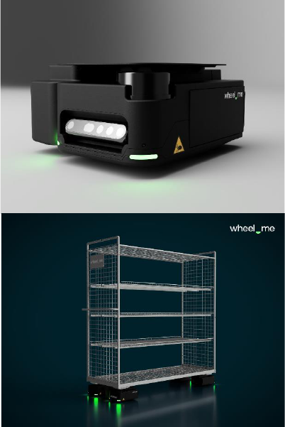
Recently, the Norwegian company wheel.me has developed
autonomous wheels. Autonomous wheels can replace regular
wheels on trolleys, carts or mounted to many other objects like
racks and pallets. They consist of computational and
mechatronic mechanisms allowing the wheels to sense the
environment, avoid collisions and drive autonomously in any
direction. Control of the wheels is done through a cloud
computing system, which can enable the coordination of
multiple objects mounted with autonomous wheels. By
mounting autonomous wheels to an object, the object can move
independently and autonomously. Autonomous wheels can be
an alternative to existing material handling equipment such as
AMRs, automated guided vehicles (AGVs), shuttles, and
conveyor belts.
Mounting autonomous wheels to storage racks removes the
need for AMRs to move racks, so in this work thanks to a long-
term collaboration between the Logistics 4.0 Lab at NTNU and
wheel.me, we have introduced and explored a new configuration
of PBS and RMF systems where we assume that loads can be
moved with autonomous wheels, extending the term loads to
include storage racks. In this way we can obtain a system with
high storage density and high throughput capacity, that we will
call Puzzle-Based Movable Rack (PBMR) system. An
illustration can be seen in Figure 1 below.
Mounting autonomous wheels to storage racks eliminates
the complexity mentioned above associated with matching
AMRs with racks and collision avoidance between unloaded
AMRs. We will assume that racks can move autonomously and
independently, thus assuming a PBMR system, where “load” is
the storage racks that can move autonomously with autonomous
wheels. Autonomous wheels also reduce constraints associated
with movement in PBS systems. Previous research in PBS
systems has mainly assumed that loads are moved with shuttles
or unit-sized conveyor belts. Under this assumption, loads have
only moved rectilinearly (i.e., in either of the four cardinal
directions) [5]. With autonomous wheels, loads can move in any
direction. Seminal research by [8] shows that travel distances
can be reduced with diagonal cross aisles in traditional aisle-
based warehouses. In our configurations, movable racks can
move also in diagonal direction.
Lastly, recent investigations of operational planning in PBS
systems indicate that retrieval time can be reduced by relaxing
constraints imposed by the original configuration [5]. By
increasing the number of escorts, it is possible to create virtual
aisles [9] allowing requested loads to move uninterruptedly. [10]
has shown through formulating an algorithm that enabled
escorts to be moved simultaneously that retrieval times could be
reduced. The term PBS system also suggests a difficult puzzle is
associated with retrieving loads. Indeed, several recent papers
propose clever algorithms for minimizing retrieval times given
constraints of the system and point to increased complexity
when the state space gets large. However, instead of taking an
operational planning perspective to solve the “puzzle” as it is, a
design optimization perspective might enable us to “cheat” the
puzzle. If it is possible to design a configuration where loads can
move diagonally to reduce travel distance and clever movement
to reduce retrieval time, there should be potential for increased
throughput capacity in a PBMR system.
Figure 1: wheel.me Genius and its installations on a movable rack.
This intersection of research topics, namely in PBS systems,
RMF systems, and non-conventional cross aisles, shapes this
work’s perspective. Description of concepts and modeling is
primarily similar to papers in the PBS research field. However,
conversely to the PBS research field, we consider density as a
result of the system configuration instead of a parameter for
operations planning and control. This perspective enables
considerably less constrained research and modeling process. It
also allows us to investigate how diagonal movement can be
utilized in a grid-based system. Most importantly, although we
do not concentrate this work on the upper limits of storage
density, we seek to find a trade-off between throughput capacity
and density, where throughput capacity can be increased from
typical PBS systems and maybe challenge RMF systems, but
with a density close to the typical PBS systems.
Specifically, we will investigate how low average cycle time
with high density can be achieved in a puzzle-based storage
system when we assume that loads can be moved with
autonomous wheels. We consider average cycle time to be the
average time needed to perform all necessary movements, which
enable a single load to be retrieved from, and a single load to be
replenished into the system. Lower average cycle time implies
higher throughput capacity for the overall system.
We divide the problem of achieving low average cycle times
into two sub-problems. First, how can we reduce average travel
distance in the system, and how can a configuration and
movement policy enable a shorter average travel distance and
movement with relaxed constraints? Travel distance is the 2-
dimensional Euclidean distance which a requested load travels
from its initially stored location to an I/O-location. The
configuration is the distribution of loads (or analogously,
escorts) according to the grid dimensions. By movement policy,
we mean the specification for performing all the necessary
movement of stored loads that enable a single load to be
retrieved from and replenished into the system.
This work seeks to meet the following objectives:
• O1. Define a travel route where loads can move diagonally
in a grid.
• O2. Design a configuration and movement policy which
retrieves requested loads along the specified travel route.
• O3. Estimate performance of a PBMR system which uses
the proposed configuration and movement policy.
This work has applied analytical modelling and simulation
approach to model a PBMR system. A program was built from
scratch as a tool to visualize and animate different
configurations and movement policies and conduct the
experiments. Furthermore, the program enabled us to assess the
feasibility of the configuration and movement policy by
simulating a large number of different cases. Given the
configuration and movement policy, we formulated an
analytical model to estimate the performance of a broader range
of scenarios than what could practically be done by the
simulation model. The analytical model has been validated
through the simulation model and both used to estimate the
performance and describe the characteristics of the
configuration and movement policy. Finally, by using the
analytical model we could compare different configurations of
the system and reflect on them for future research.
The main contributions of this work are:
1 A puzzle-based moveable rack (PBMR) system with
autonomous wheels is proposed.
2 This work is the first to propose a configuration that
enables diagonal movement that can save travel
distance up to 18.7% compared to the orthogonal (or
Manhattan) distances.
3 We combine simultaneous movement and block moves
with virtual aisles in a configuration and movement
policy that enables the requested load to be retrieved
uninterruptedly. As a result, the configuration and
movement policy can achieve an average cycle time
that is practically only dependent on average travel
distance and not constrained by the movement of non-
requested loads.
II. ANALYTICAL MODELLING AND SIMULATION
We use the following assumptions in order to model the
operation of the PBMR and so estimated the travel distance and
the travel time.
We assume that loads in the system are moved with
autonomous wheels, and the autonomous wheels operate
without errors. As mentioned, with this assumption, we expand
the term “loads” to also encapsulate storage racks in addition to
totes, pallets, containers, and other units previously
encapsulated by this term in the literature about PBS systems.
Although movement with autonomous wheels is not constrained
to a physical grid such as movement with shuttles or unit-sized
conveyor belts, we use an imaginary grid to model layout design
and behavior. This choice implies that layout design and
behavior will be similar and use many of the same theoretical
concepts as PBS systems.
Each load resemble one storage rack which can move with
autonomous wheels (1 m/s). Time required to change direction
is neglected. The storage area is modelled as a discrete grid with
cell dimensions of 1m x 1m. An escort move changes the
location of an escort from its initial cell to a new cell by moving
the load(s) between the two locations. Each moved load is a
consequence of an escort move. From each cell, a load can be
moved to either of its eight adjacent cells. A load can move to
either of the four adjacent cells in the same row or column, or it
can move to either of the four adjacent cells in the diagonal
directions. Loads are requested from a uniform distribution.
Single command operations, commonly termed single load
retrieval in PBS systems literature.
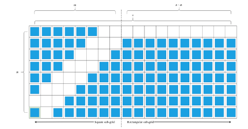
Each shape can be modelled with square and a rectangular
sub-grids (Fig. 2). The operations in the square and rectangular
sub-grids were implemented in an object oriented program
written in Python 3.6 in order to validate the results of the
analytical model. m and n are the two side of the grid. Where (m,
m) are the dimensions of the square sub-grid, and (m, n-m) are
the dimensions of the rectangular sub-grid.
Figure 2: A rectangular grid divided into a square and a rectangular sub-grid
Regarding the movement policy, for any diagonal
movements, we can use a pseudo-straight route as the shortest
route since the route resembles the straight line between the cell
at (i, j) and the I/O-location and it can be modelled as sum of a
rectilinear movement and a diagonal movement in the square
sub-grid. It is easy to see from Figure 3 that, in fact, both routes
have equal route lengths. Moreover, the number of colored cells
is equal to the Chebyshev distance between the two cells.
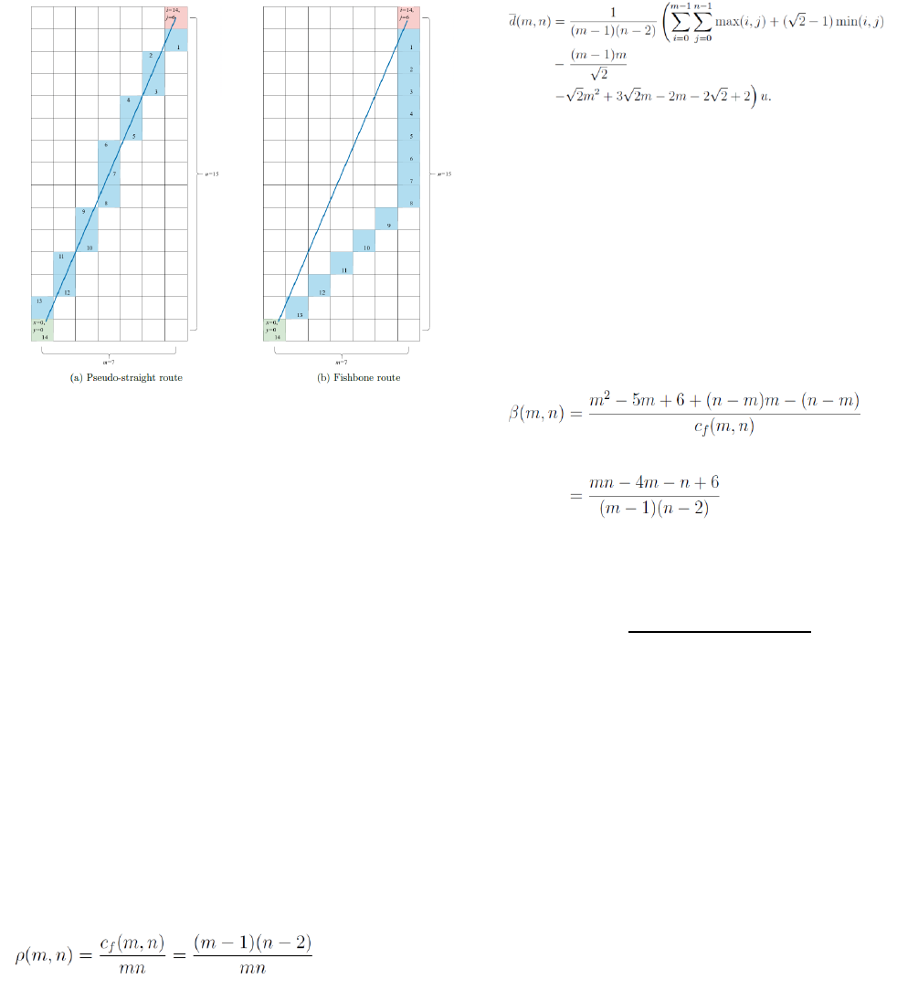
Figure 3: Converting Psuedo-straight route to Fishbone route
In a generic grid, to move a load to I/O-location, in the
rectangular sub-grid, an empty aisle for the rectilinear
movement needs to be created (if the load is in a that sub-grid).
Then the load can be move to the side closest to the square sub-
grid where I/O is located. As soon as in the square sub-grid (or
if the load is already located in that sub-grid) there will be other
rectilinear movement (also in that case the empty aisle need to
be created) to enter the diagonal aisle of the square sub-grid and
then finally the diagonal movement to I/O-location.
Some movements can be synchronized, so the creation of
empty aisle and the movement of the load can be performed
sequentially or fully simultaneously.
Based on the assumptions and the movement policy
described here above, we developed some analytical models for
density, travel distance and travel time, considering different
configurations.
A. Density
Density for an m x n grid is modeled as the capacity divided
by the grid size. Grid size is the total number of cells in the grid,
while we need to leave an empty aisle for the diagonal of the
square sub-grid and an empty rectilinear aisle for the rectangular
sub-grid. So the density is expressed as (1):
(1)
B. Average travel distance
Average travel distance for an m x n grid is modeled based
on the potential diagonal movement as follows, where i and j are
the coordinates of the analysed cell and u is the length of the
sides of the cell in meters (in our study is 1m)
(2)
C. Average cycle time
The average cycle time needs to consider the time necessary
to create the empty aisle. In fact some loads need to wait for one
step for a rectilinear aisle to be opened before they can be
escorted to the IO-location. For these loads, this is the only
additional step beside the steps needed to transport the load to
the IO-location. The number of loads in the grid that require an
additional step to open a rectilinear aisle can be represented as a
fraction of all loads in the grid, β(m, n). The loads that require
an additional step are all the loads that are not next to the
diagonal aisle:
(3)
The average cycle time is so the additional time added to the
average travel time:
(4)
Where β(m, n)/v (we called βv) can be interpreted as the
average time used to move non-requested loads and d(m, n)/v
(we called dv) can be interpreted as the average travel time of
the requested loads.
III. RESULTS AND DISCUSSION
We run different scenarios characterized by different
configurations. First with square shape and grid size from 0 to
2130 m². Then we considered rectangular shapes with different
ratio r = n/m, in particular 2, 3, and 4. We considered 1 I/O-
location as initial configuration and then we extended it to 2, 3
and 4.
First, we validated the analytical model with the results
obtained by the simulation for a shape ratio of 1. The accuracy
of the analytical model is promising with an error of about 2%.
We can see also that the additional time β is about 5% of total
time. Next, we can also observe that the average cycle time
follows a similar square root increase as the average travel
distance. The average cycle time can be decomposed into two
contributions, the time it takes for the requested load to travel
the average travel distance, the travel time, denoted dv, and the
extra time required to clear the way for the requested load,
denoted βv. Analytical and simulated average cycle time is
plotted together with analytical travel time dv and βv. Both βv
and average travel distance increase for increasing grid size, but
it is obvious how the extra time needed to open the rectilinear
(, ) =
((, ) +
(, ))
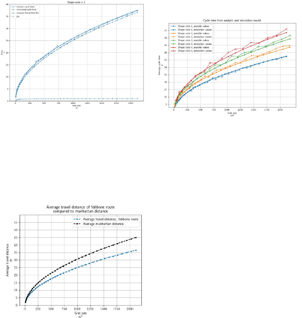
aisle is very small compared to the average travel time and
practically constant. For grids bigger than 225m², βv only ranges
between 0.86 seconds to 0.95 seconds, whereas average travel
time closely follows the same square root increase as the
analytical and simulated cycle time. Therefore, the average
cycle time is mostly dependent on the average travel time and
not the time of moving other loads.
Figure 4: Analytical model and simulation model for average cycle time.
Then we estimated the advantage to use diagonal movements
compared to traditional Manhattan ones in a squared grid (shape
ratio = 1) (fig. 5). The average Manhattan distance for a grid
with a size of 2116m2 is 45m, whereas the average travel
distance of our configuration and movement policy is 36.6m.
Overall, considering the different sizes, there is about 15% to
19% reduction in average travel distance compared to the
Manhattan distance. In general the average travel distance of the
fishbone route seems to follow a square root increase when the
grid size increase.
Figure 5: Average travel distance of Fishbone compared to Manhattan for shape
ratio = 1 – squared shape.
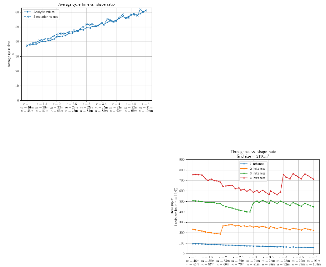
Average cycle times of four different shape ratios are
combined in in Figure 6. Possible configurations of m × r*n is
more sparsely distributed over grid sizes for increasing shape
ratio. This is why the number of points on each plots linearly
declines for increasing r. Average cycle time increases more
rapidly for larger shape ratios, with a simulated maximum of
37.34 seconds for the grid with r = 1 and a simulated maximum
of 55.99 seconds for the grid with r = 4 for the same grid size,
2116m². This is a 50.0% relative increase in average cycle time
from shape ratio r = 1 to r = 4.
Figure 6: Average cycle time for different shape ratios (both analytical and
simulation models)
Change in average cycle time can be further investigated by
studying average cycle time for varying shape ratios. Figure 7
illustrates how average cycle time increases close to linearly
relative to the shape ratio. In this experiment, a fixed target grid
size is set to be 2130m², which was the maximum grid size of
the previous experiment. Since n and m must be integers, the
actual grid sizes deviate slightly for different size ratios, namely
SD=46,67 cells (= 2.14% relative standard deviation) for shape
ratios in the range 1 to 5. All grid sizes are within 4.74% of
2130m², yielding an average capacity of 2000 loads (SD=43,3
loads). The simulated average cycle time has a relative increase
of 63.7% from average cycle time of 37.34s when r = 1, to
average cycle time of 61.14s when r = 5. Again, by decomposing
the average cycle time, we can observe that the average travel
distance closely follows the average cycle time. The average
travel distance is 36.6m when r = 1, and 60.1m when r = 5.
However, the reduction in travel distance is only 3.1% compared
to the Manhattan distance when r = 5. This quick reduction in
improvement is because the angle of the diagonal aisle is always
45 degrees. Consequently, when the grid dimensions get more
skewed, travel along the diagonal aisle compared to rectilinear
aisles is lower, and the contribution of reduced travel distance is
less significant. Intuitively, when the grid dimensions get more
skewed, both the average Manhattan distance and the fishbone
route length get closer to the Euclidean distance because one
component of the travel route gets significantly longer than the
other. Nevertheless, to get the shortest average cycle time and
the biggest reduction in average travel distance compared to
Manhattan distance, grid dimensions should have a shape ratio
close to r = 1.
Figure 7: Average cycle time varying shape ratios (both analytical and
simulation models)
Number of I/O-locations has a great impact, but it depends
how square the total grid is and how many squared sub-grids can
be created based on the available I/O-locations
The analytical model has been used to estimate the
theoretical throughput of the grid configuration and movement
policy. In Figure 8 throughput for combinations of 1, 2, 3, and 4
I/O-locations is plotted for increasing shape ratio. This is the
inverse of the average cycle time from the last experiment
depicted in previous figures. The other grids have configurations
varying according to shape ratio as described in previous
sections. When a grid can consist only of I/O-location, the
maximum throughput is achieved when r = 1 with 95,9 loads per
hour. For grids consisting of 2, 3 and 4 I/O-locations, maximum
throughput is 274.8, 510.5, and 764 loads per hour at shape
ratios r = 2.2 r = 3.3 r = 4.3 respectively.
Naturally, throughput is higher for grids with more I/O-
locations, but the difference is not constant. Whereas throughput
of grids with a single I/O-location steadily declines for
increasing r, grids with combinations of instances experience
jumps in throughput for specific values of r. This behavior is a
consequence of how the I/O-locations are combined for different
grids and the effect of different shape ratios. With the specified
combination of grids, the throughput of the grids in this
experiment depends on two factors. The number of I/O-locations
is one obvious factor, but this is constant for increasing shape
ratio. The second factor is the average travel distance of each
individual instance in a grid, which does vary with the shape
ratio. For shape ratios greater or equal to the number of I/O-
locations, grids can suddenly be combined of I/O-locations with
individual shape ratios r = 1. As illustrated in the previous
scenario, grids with shape ratios closer to 1 have shorter average
travel distance and shorter average cycle time, thus increasing
throughput.
Moreover, before r is equal to the number of instances, a
relatively quick decline in throughput is noticeable for grids
consisting of 2, 3, and 4 I/O-locations compared to 1 I/O-
location. The relatively quick decline in throughput occurs
because the shape ratios of the individual I/O-location increase
more rapidly when the grid is divided into several I/O-locations
compared to one. This behavior stops when the shape ratio is
greater or equal to the number of I/O-locations in each grid,
where a less steep decline occurs.
Another pattern is noticeable when the shape ratio is greater
than the number of I/O-locations. Oscillations in throughput
occur in all grids for larger shape ratios. (This is easy to see from
Figure 8 for grids with 2, 3, or 4 I/O-locations, but also occurs
in grids with single I/O-locations as can be seen more easily in
Figure 7). Furthermore, the oscillations are larger for grids
consisting of more I/O-locations. The oscillations are also due
to variations in average travel distance for individual I/O-
locations, but more specifically, it is because the I/O-locations
must increase dimensions in incremental steps. In grids with
more I/O-locations, the effect is more drastic. The small spikes
occur whenever m is reduced by one. This pattern also occurs
when the shape ratio is less than four for grids consisting of four
I/O-locations. Since decrements in the shortest side occur more
frequently for smaller shape ratios, an oscillation occurs for
every change in shape ratio when 2.5 ≤ r ≤ 3.3.
Figure 8: Throughput vs shape ratio, varying the number of I/O-locations
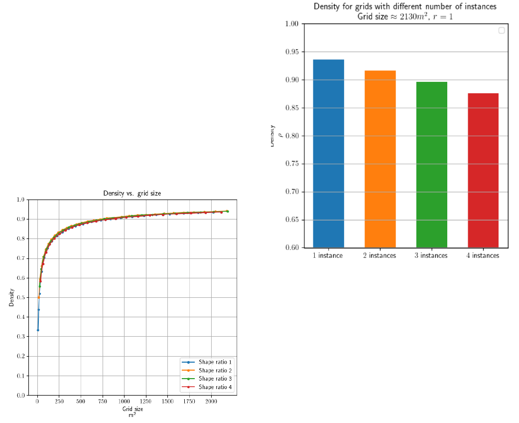
Densities for grids with different shape ratio all increase very
similarly with increasing grid size, as can be seen in Figure 5.5.
All grids reach a density over 0.9 when the grid size passes
841m² and reaches a maximal density of approximately 0.94 for
the maximal grid size.
Whereas the relative increase in average cycle time is 50.0%
for the biggest two grids with shape ratios 1 and 4, the density is
identical for both grids. The density for both grids with r = 1 and
r = 4 is 0.936 when the grid size is 2116m². Figure 9 shows how
densities in addition to being very similar for all shape ratios, are
practically identical for grids with shape ratio r = 1 and r = 4 for
all grid sizes. This similarity in density might seem
counterintuitive since a square grid requires escorts to make a
diagonal aisle, and a diagonal aisle requires more escorts than a
rectilinear aisle for aisles of the same length.
A grid with r = 4 needs mostly escorts to make a rectilinear
aisle, but a rectilinear aisle in this grid is relatively long
compared to the grid size. To be precise, the rectilinear aisle is
three times longer than the diagonal aisle when r = 4 and one
needs three escorts for every cell on the diagonal path to make a
diagonal aisle. Lastly, the diagonal path is twice as long for grids
with r = 1 compared to grids with r = 4. That is why the densities
are practically identical for grids with r = 1 and r = 4. Grids with
r = 2 and r = 3 achieve slightly higher densities but only a relative
increase of 0.4%.
To summarize, density is practically unaffected by shape
ratio, but shape ratio is a significant parameter for average travel
distance, and consequently, average cycle time.
Figure 9: Density vs grid size, varying the shape ratio
The previous scenario where a grid with a single I/O-location
is analyzed illustrates how density is practically independent of
shape ratio.
We can see how this is analogously transferrable to grids
consisting of multiple I/O-locations by observing how the
average density for grids consisting of 1, 2, 3 or 4 I/O-locations
is 0.938, 0.915,0.895, and 0.875 with minimal standard
deviations 0.002, 0.002, 0.005, and 0.006 respectively.
The difference in densities for the different number of I/O-
location in a grid occurs because each I/O-location needs an
independent set of escorts. The relative reduction in density is
only 6% from grids consisting of only one I/O-location to four
ones. Densities for grids consisting of the different number of
I/O-locations are plotted in Figure 10.
Figure 10: Density vs I/O-locations
IV. CONCLUSION AND FUTURE RESEARCH
Since Logistics 4.0 Lab (NTNU) started the collaboration
with wheel.me on the use of autonomous wheels in
intralogistics, the research team conceptualized a potential
application of the autonomous wheels to warehousing
applications.
By mounting autonomous wheels to an object, the object can
move independently and autonomously in any direction. So we
created a PBS system with movable racks, called Puzzle-Based
Movable Rack (PBMR) system, so reaching high density and
high throughput performance, even more exploiting the diagonal
movements.
We developed an analytical model for a modular
representation of the system, composed by square and
rectangular sub-grids, and we validated it with simulation.
We demonstrated the high density (around 90-95%) and
higher throughput compared to Manhattan movements (+ about
18%). We also investigated the implications of different
configurations, like varying the shape ratio and the number of
I/O-locations.
This is the first research investigating such system, so future
research is needed and they should focus first on the extension
of the analysis with more study on optimal design of such
system, considering also different storage policies. When design
guidelines have been introduced, research should focus on the
operational aspects of such system, studying for example the
sequencing of loads, the allocation of escorts, the allocation of
I/O-location. In both cases, design related and operational
related, multi-objective optimization or analysis should be
implemented in order to give practical implications to managers
when it comes to find the proper trade-off between density and
throughput.
Finally real testing and first implementation would be
needed to validate the results also in real operational conditions.
REFERENCES
[1] Boysen, N., De Koster, R., & Weidinger, F. (2019). Warehousing in the
e-commerce era: A survey. European Journal of Operational Research,
277(2), 396-411.
[2] Gue, K. R., & Kim, B. S. (2007). Puzzle‐based storage systems. Naval
Research Logistics (NRL), 54(5), 556-567
[3] Wurman, P. R., D'Andrea, R., & Mountz, M. (2008). Coordinating
hundreds of cooperative, autonomous vehicles in warehouses. AI
magazine, 29(1), 9-9.
[4] Azadeh, K., De Koster, R., & Roy, D. (2019). Robotized and automated
warehouse systems: Review and recent developments. Transportation
Science, 53(4), 917-945.
[5] Raviv, T., Bukchin, Y., & de Koster, R. B. M. (2023). Optimal Retrieval
in Puzzle-Based Storage Systems Using Automated Mobile Robots.
Transportation Science, 1-20.
[6] Gharehgozli, A., & Zaerpour, N. (2020). Robot scheduling for pod
retrieval in a robotic mobile fulfillment system. Transportation Research
Part E: Logistics and Transportation Review, 142, 102087.
[7] Keung, K. L., Lee, C. K., Ji, P., & Ng, K. K. (2020). Cloud-based cyber-
physical robotic mobile fulfillment systems: A case study of collision
avoidance. IEEE Access, 8, 89318-89336.
[8] Gue, K. R., & Meller, R. D. (2009). Aisle configurations for unit-load
warehouses. IIE transactions, 41(3), 171-182.
[9] Gue, K. R., Furmans, K., Seibold, Z., & Uludağ, O. (2013). GridStore: a
puzzle-based storage system with decentralized control. IEEE
Transactions on Automation Science and Engineering, 11(2), 429-438.
[10] Yu, Y., Yu, H., De Koster, R., & Zaerpour, N. (2017). Optimal algorithm
for minimizing retrieval time in puzzle based storage system with multiple
simultaneously movable empty cells. Working Paper Erasmus University,
Rotterdam.
